New Semester Started Get 50% OFF Study Help! --h --m --s Claim Now

Question Answers

Textbooks

Find textbooks, questions and answers

Oops, something went wrong!

Change your search query and then try again

Result Not Found

Books FREE
Study Help
Tutors
AI Study Planner NEW
Sell Books

Search
Sign In
Register

study help
business
introduction to probability statistics

Probability And Statistics For Engineers 9th Global Edition Richard Johnson, Irwin Miller, John Freund - Solutions

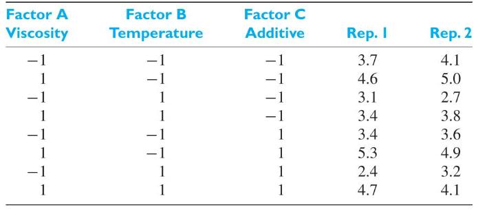
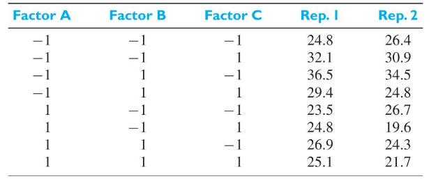
The effect on engine wear of oil viscosity, temperature, and a special additive was tested using a \(2^{3}\) factorial design. Given the following results from the experiment,Interpret the effects based on the confidence intervals. Factor A Viscosity 1 Factor B Temperature Factor C Additive Rep. I
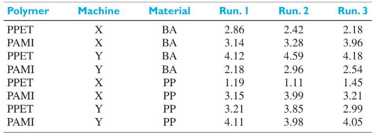
Two machines \(X\) and \(Y\) were used to produce two types of plastic polymers, PPET and PAMI. The polymers were produced using materials BA and PP. The production was run 3 times. The \(y\) values given below are the logarithms of the quantity of polymers produced.Analyze this experiment using
The response variable \(Y_{i j}\) in a \(2^{2}\) design can also be expressed as a regression model\[Y_{i j}=\mu+\beta_{1} x_{1}+\beta_{2} x_{2}+\beta_{12} x_{1} x_{2}+\varepsilon_{i j}\]where the \(\varepsilon_{i j}\) are independent normal random variables and each has mean 0 and variance
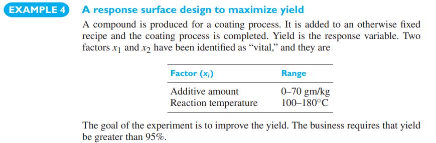
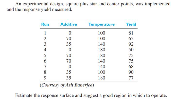
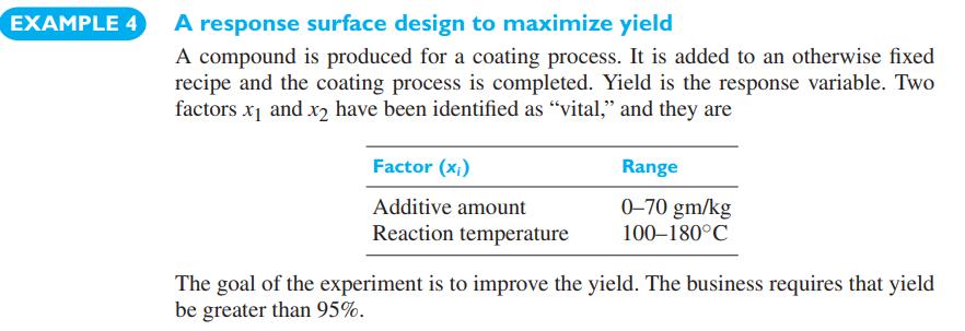
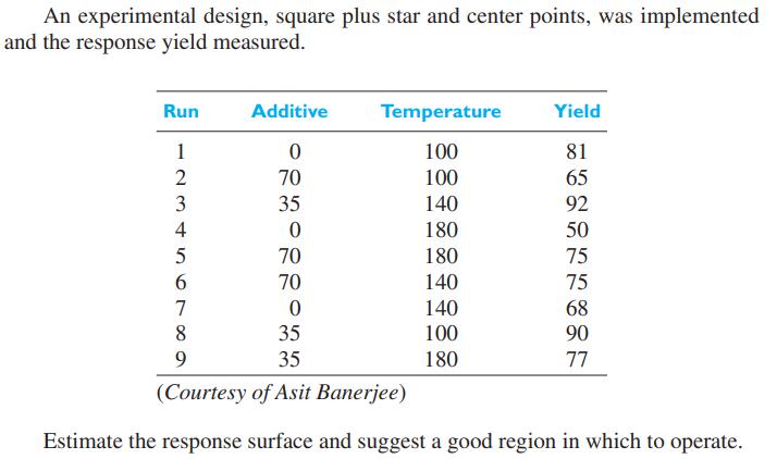
Refer to the Example 4. Use calculus to obtain the location of the estimated maximum yield when all terms are included in the model.Data From Example 4 EXAMPLE 4 A response surface design to maximize yield A compound is produced for a coating process. It is added to an otherwise fixed recipe and
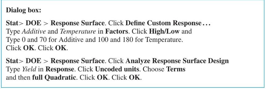
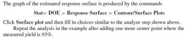
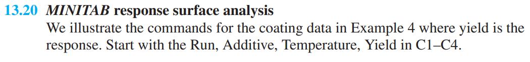
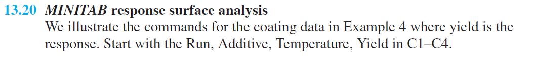
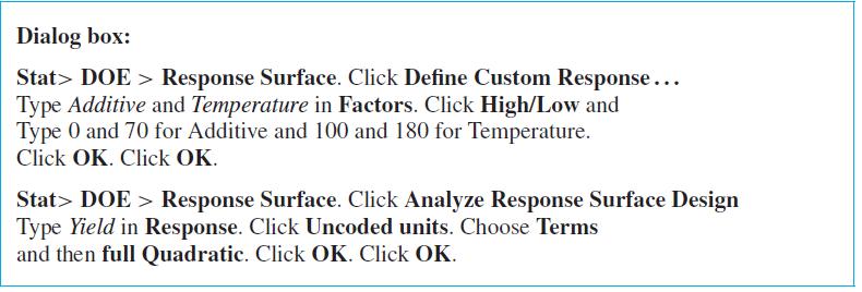
MINITAB response surface analysis We illustrate the commands for the coating data in Example 4 where yield is the response. Start with the Run, Additive, Temperature, Yield in C1-C4. Dialog box: Stat> DOE Response Surface. Click Define Custom Response... Type Additive and Temperature in Factors.
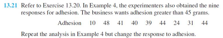
Refer to Exercise 13.20. In Example 4, the experimenters also obtained the nine responses for adhesion. The business wants adhesion greater than 45 grams.\[\begin{array}{llllllllll} \text { Adhesion } & 10 & 48 & 41 & 40 & 39 & 44 & 24 & 31 & 44
Is there a region within the experimental region where estimated adhesion is greater than 45 grams? Construct a contour plot to show this region. Note that MINITAB does keep nonsignificant terms. Refer to Exercise 13.21.Data From Exercise 13.21Data From Example 4 13.21 Refer to Exercise 13.20. In
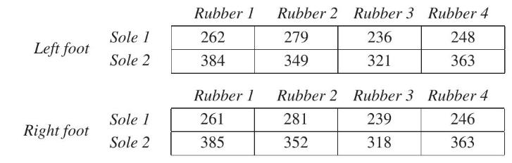
A footwear manufacturing machine manufactures each piece separately. Suppose pairs are manufactured, with the following results obtained for the range (number).Perform an appropriate analysis of variance, and test for the presence of an interaction. Rubber 1 Rubber 2 Rubber 3 Rubber 4 Sole 1 262
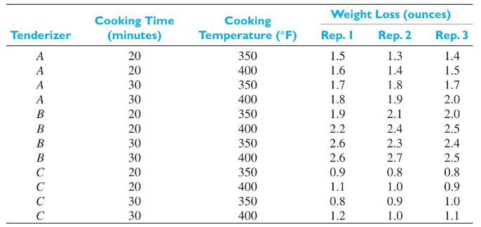
A study was conducted to measure the effect of 3 different meat tenderizers on the weight loss of steaks having the same initial (precooked) weights. The effects of cooking temperatures and cooking times also were measured by performing a \(3 \times 2 \times 2\) factorial experiment in 3
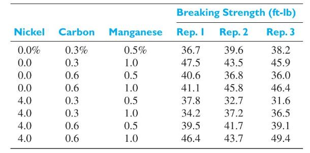
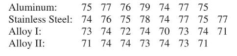
An experiment was conducted to determine the effects of certain alloying elements on the ductility of a metal, and the following results were obtained:Perform an appropriate analysis of variance and interpret the results. Breaking Strength (ft-lb) Nickel Carbon Manganese Rep. I Rep. 2 Rep. 3 0.0%
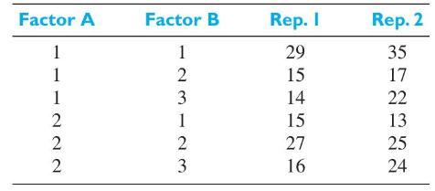
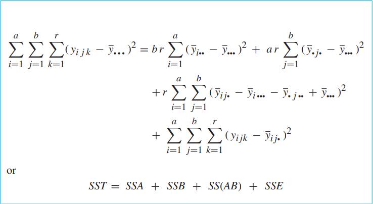
Given the two replicates of a \(2 \times 3\) factorial experiment, calculate the analysis of variance tables using the formulas on page 428 .Data From page 428 Factor A Factor B Rep. I Rep. 2 1 1 12 1 29 35 2 15 17 1 3 14 22 222 2 123 15 13 27 25 16 24
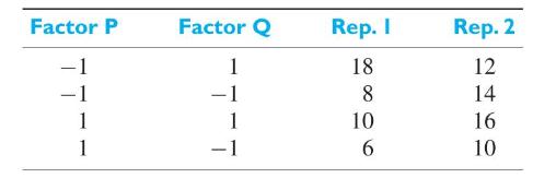
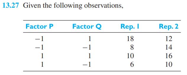
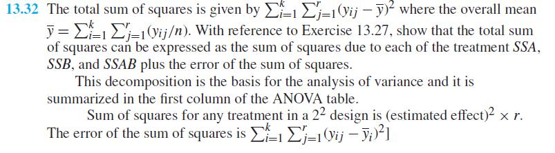
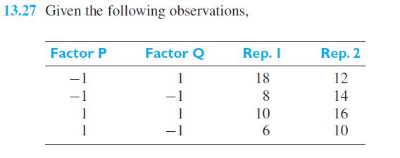
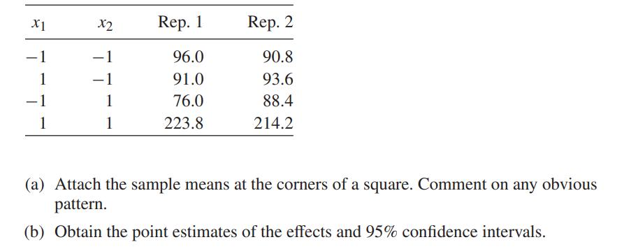
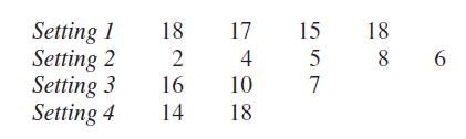
Given the following observations,Interpret the effects based on the confidence intervals. Factor P Factor Q Rep. I Rep. 2 1 18 12 -1 8 14 1 1 1 10 16 - 6 160 10
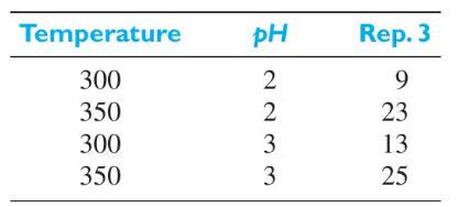
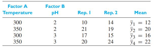
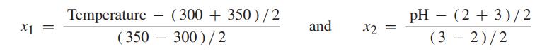
With reference to the example on page 443, suppose a third replicateis run. Analyze the experiment, using all 3 replicates, according to the visual procedure given in Section 13.3. Interpret the effects based on the confidence intervals.Data From Page 443 Temperature pH Rep. 3 300 350 300 350
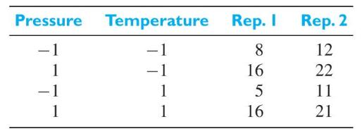
Trouble was being experienced by a new high-tech machine for joining two pieces of sheet metal. The two factors considered first are the pressure (low/high) and temperature of the pump low/high. The response is the diameter \((\mathrm{mm})\) of a button-shaped joint which is an indirect measure of
A computer engineer studied the working of a motherboard under different conditions. The response is heating effect (coded units). The factors are fan connectors (no. of pins), power connection (type), and chipsets (direction).Interpret the effects based on confidence intervals. Factor A Factor B
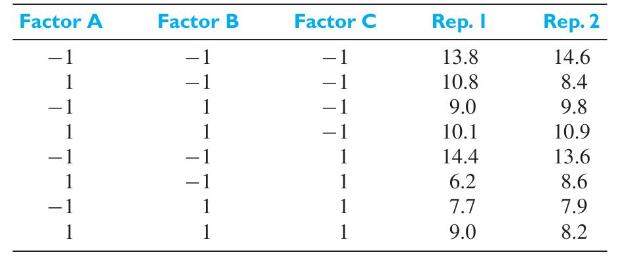
Given the following results from a \(2^{3}\) factorial experiment,Interpret the effects based on the confidence intervals. Factor A Factor B Factor C Rep. I Rep. 2 -1 13.8 14.6 10.8 8.4 1 9.0 9.8 1 10.1 10.9 1 14.4 13.6 1 6.2 8.6 1 7.7 7.9 9.0 8.2
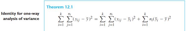
The total sum of squares is given by \(\sum_{i=1}^{k} \sum_{j=1}^{r}\left(y_{i j}-\bar{y}\right)^{2}\) where the overall mean \(\bar{y}=\sum_{i=1}^{k} \sum_{j=1}^{r}\left(y_{i j} / n\right)\). With reference to Exercise 13.27, show that the total sum of squares can be expressed as the sum of
With reference to the example of the \(2^{3}\) design on page \({ }^{* * *}\), express the total sum of squares as the sum of the contributions from each of the seven treatments plus the error sum of squares.This decomposition is the basis for the analysis variance and it is summarized in the first
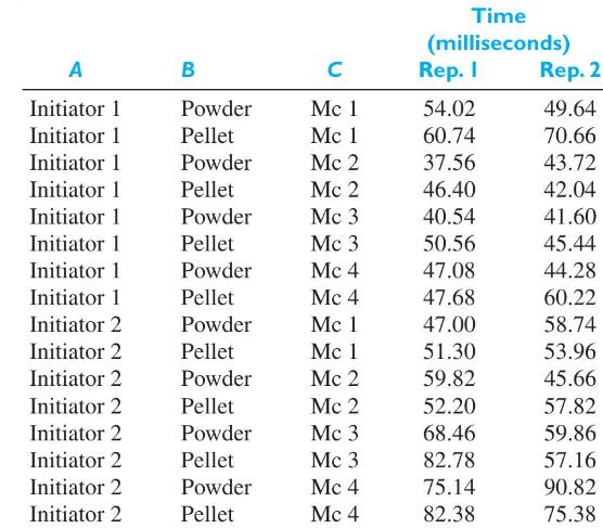
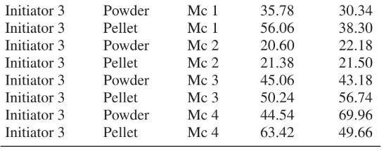
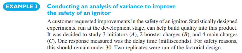
With reference to the Example 3 concerning improvements in the safety of an ignitor, the time to reach maximum pressure was also recorded. Two replicates were run of the factorial design and the times to reach maximum pressure recorded. Analyze the results of this experiment.Data From Example
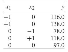
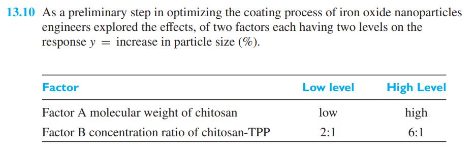
Refer to Exercise 13.10 where the response is \(y=\) increase in particle size. Besides the first replicate, the investigators also performed the experiments that form the star part of the design.Using all 9 measurements, fit a response surface as in Example 4.Data From Exercise 13.10Data From
In a factory, 20 observations of the factors that could heat up a conveyor belt yielded the following results:0.36,0.41,0.25,0.34,0.28,0.26,0.39,0.28,0.40,0.26,0.35,0.38,0.29,0.42,0.37,0.37,0.39,0.32,0.29 and 0.36 . Use the sign test at the 0.01 level of significance to test the null hypothesis
The time sheet of a factory showed the following sample data (in hours) on the time spent by a worker operating a hydraulic gear lift: 1.0,0.8,0.5,0.9,1.2,0.9,1.4,10,1.3,0.8,1.5,1.2,1.9,1.1,0.7,0.8,1.1,1.2, 1.5,1.1,1.8,0.5,0.8,0.9, and 1.6. Use the sign test at the 0.05 level of significance to
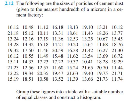
With reference to Exercise 2.12, which pertained to the particle size of cement dust in a factory producing cement, use the sign test at the 0.05 level of significance to test the null hypothesis \(\tilde{\mu}=15.13\) hundredth of a micron against the alternative hypothesis \(\tilde{\mu}Data From
The following are the number of classes attended by 2 students on 20 days: 3 and 5, 1 and 2, 3 and 4, 2 and 5, 5 and 3, 4 and 2, 1 and 3, 1 and 4, 1 and 2, 2 and 4, 3 and 2, 2 and 5, 5 and 5,1 and 3,2 and 4, 2 and 2, 2 and 3,3 and 5, 3 and 3,2 and 1 . Use the sign test at the 0.01 level of
Comparing two types of automobile engines, a consumer testing service obtained the following pickup ( \(0-100 \mathrm{kmph})\) times (rounded to the nearest tenth of a second):Use the \(U\) test at the 0.05 level of significance to check whether it is reasonable to say that the population of pickup
The following are the self-reported times (hours for month), spent on homework, by random samples of juniors in two different majors.Use the \(U\) test at the 0.05 level of significance to test whether or not students from the 2 groups devote the same amounts of time to homework. Major 1: 63 72 29
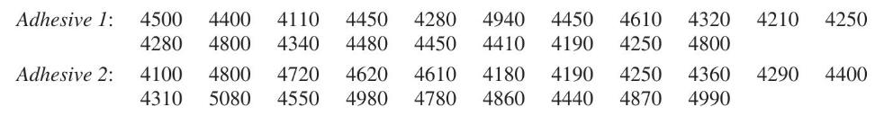
The following are the data on the strength (in psi) of 2 kinds of adhesives:Use the \(U\) test at the 0.01 level of significance to test the claim that the strength of Adhesive 1 is stochastically larger than the strength of Adhesive 2. Adhesive 1: 4500 4400 4110 4450 4280 4800 4340 Adhesive 2:
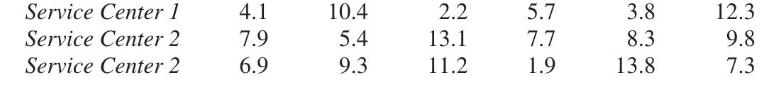
A company that processes health claims maintains three centers. Software was installed so they could monitor non-business internet usage by their employees. Initially, six employees were randomly selected from each of three service centers and the number of hours of non-business internet usage
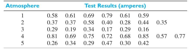
So-called Franklin tests were performed to determine the insulation properties of grain-oriented silicon steel specimens that were annealed in five different atmospheres with the following results:Use the \(H\) test at the 0.05 level of significance to decide whether or not these 5 samples can be
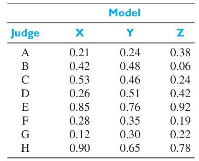
A panel of 8 judges was asked to rate each of 3 models developed by engineering students on the likelihood that these models can be practically implemented to harness the controlled fusion energy. Their ratings (in the form of judgmental probabilities) are as follows:Calculate the rank correlation
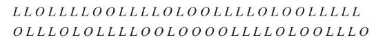
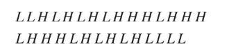
The following arrangement indicates whether 60 consecutive cars which went by the toll booth of a bridge had local plates, \(L\), or out-of-state plates, \(O\) :Test at the 0.05 level of significance whether this arrangement of \(L\) 's and \(O\) 's may be regarded as random.
The following are the graded scores (out of 20) obtained by a class of 28 students in statistics: 12,8,6,10,9,15,18,19,20,18,20,16,12,10,14,16,17,19,20,20,14,11,12,15,17,16,12, and 17. Test for randomness at the 0.05 level of significance.
The following are 42 consecutive pizza breads baked by a newly improved oven model during 6 weeks:25,28,32,31,30,29,16,18,31,24,72,55,61,33,30,44,46,59,62,75,75,80,70,64,48,52,39,38,61,64,38,48,35,34,49,58,63,36,75,80,32, and 48 . Use the method of runs above and below the median and the 0.01 level
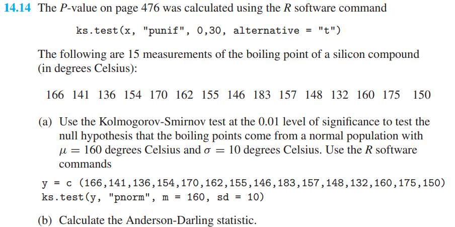
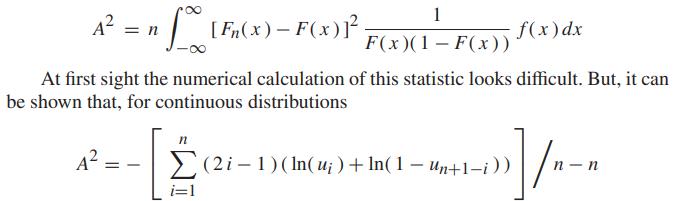
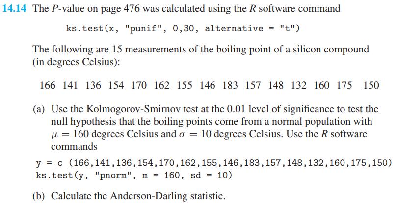
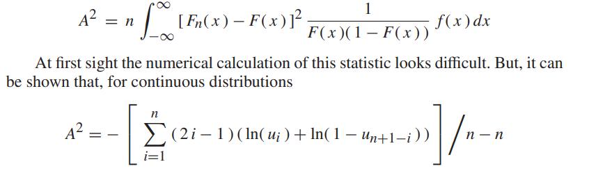
The \(P\)-value on page 476 was calculated using the \(R\) software command ks.test(x, "punif", 0,30 , alternative \(=\) "t")The following are 15 measurements of the boiling point of a silicon compound (in degrees Celsius):\[\begin{array}{lllllllllllllll} 166 & 141 & 136 & 154 & 170
In a vibration study, certain airplane components were subjected to severe vibrations until they showed structural failures. Given the following failure times (in minutes), test whether they can be looked upon as a sample from an exponential population with the mean \(\mu=10\)
According to Einstein's theory of relativity, light should bend when it passes through a gravitational field. This was first tested experimentally in 1919 when photographs were taken of stars near the sun during a total eclipse and again when the sun had moved to another part of the sky. These
Referring to Exercise 12.6, use the \(U\) statistic at the 0.05 level of significance to test whether weight loss using lubricant A tends to be less than the loss using lubricant \(\mathrm{B}\).Data From Exercise 12.6 12.6 With reference to the example on page 389, suppose one additional
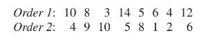
To find the best order of tools on a factory workbench, two different orders were compared by simulating an operational condition and measuring the response time taken to respond to the condition change. The response time (in minutes) of 16 engineers (randomly assigned to the two different orders)
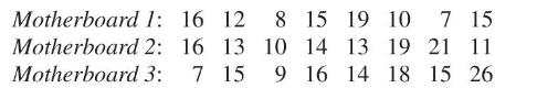
The following are the data on time taken by a computer engineer to assemble 8 computers each for 3 types of mother boards.Use the \(H\) test at the 0.05 level of significance to test whether there is a difference in the assembly times of the three types of motherboards. Motherboard 1: 16 12
To test whether radio signals from deep space contain a message, an interval of time could be subdivided into a number of very short intervals and it could then be determined whether the signal strength exceeded a certain level (background noise) in each short interval. Suppose that the following
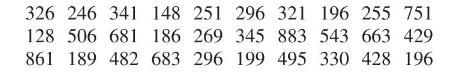
The total number of vehicles crossing a toll booth each day during the month of November were:Making use of the fact that the median is 328 , test at the 0.01 level of significance whether there is a significant trend. 326 246 341 148 251 296 321 196 255 751 128 506 681 186 269 345 883 543 663 429
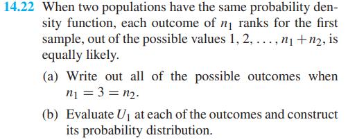
When two populations have the same probability density function, each outcome of \(n_{1}\) ranks for the first sample, out of the possible values \(1,2, \ldots, n_{1}+n_{2}\), is equally likely.(a) Write out all of the possible outcomes when \(n_{1}=3=n_{2}\).(b) Evaluate \(U_{1}\) at each of the
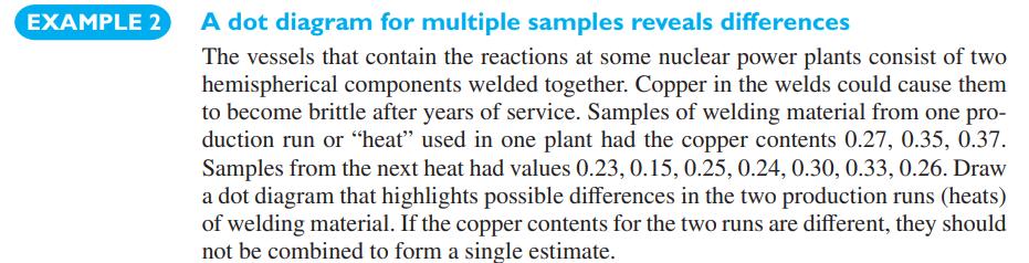
With reference to Example 2, Chapter 2, use the \(U\) statistic to test the null hypothesis of equality versus the alternative that the distribution of copper content from the first heat is stochastically larger than the distribution for the second heat. Following the approach in Exercise 14.22, it
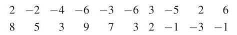
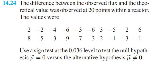
The difference between the observed flux and the theoretical value was observed at 20 points within a reactor. The values wereUse a sign test at the 0.036 level to test the null hypothesis \(\tilde{\mu}=0\) versus the alternative hypothesis \(\tilde{\mu} eq 0\). 2-2-4-6-3 -6 3-5 26 -63-526 28 -3-1
With reference to Exercise 14.24, test for randomness with level 0.05 .Data From Exercise 14.24 14.24 The difference between the observed flux and the theo- retical value was observed at 20 points within a reactor. The values were 2-2-4-6-3-63-5 26 85 3 9 7 32-1-3-1 Use a sign test at the 0.036
Survival times (days) of fuel rods in a nuclear reactor are as follows:Test at the 0.01 level of significance whether these data are consistent with the assumption of a log-normal distribution of survival times. Use the Kolmogorov-Smirnov test and see Exercise 14.14.Data From Exercise 14.14 16 11
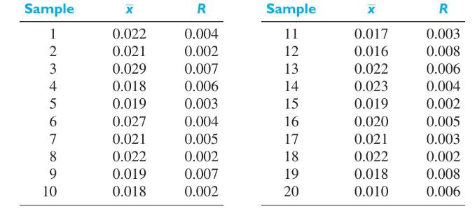
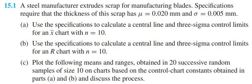
A steel manufacturer extrudes scrap for manufacturing blades. Specifications require that the thickness of this scrap has \(\mu=0.020 \mathrm{~mm}\) and \(\sigma=0.005 \mathrm{~mm}\).(a) Use the specifications to calculate a central line and three-sigma control limits for an \(\bar{x}\) chart with
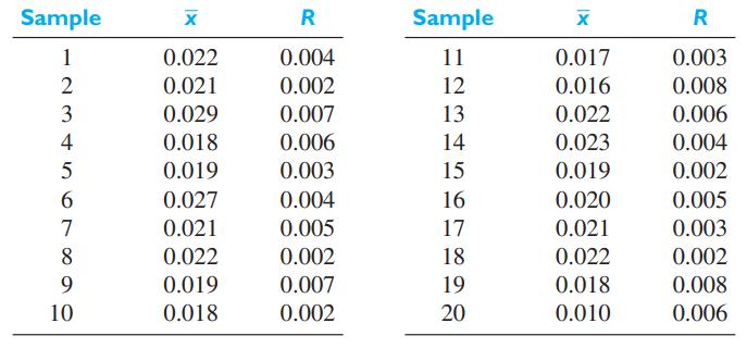
Calculate \(\overline{\bar{x}}\) and \(\bar{R}\) of the data of part (c) of Exercise 15.1, and use these values to construct the central lines and three-sigma control limits for new \(\bar{x}\) and \(R\) charts to be used in the control of the thickness of the scrap steel.Data From Exercise 15.1
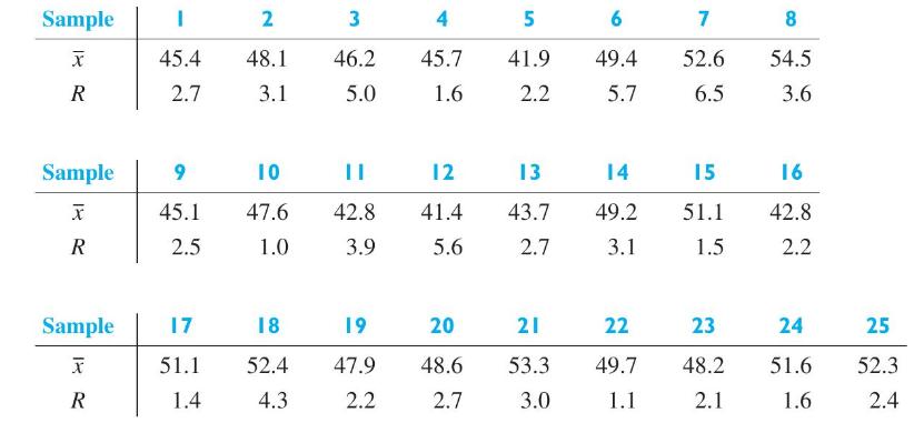
The following data give the means and ranges of 25 samples, each consisting of 4 compression test results on steel forgings, in thousands of pounds per square inch:(a) Use these data to find the central line and control limits for an \(\bar{x}\) chart.(b) Use these data to find the central line and
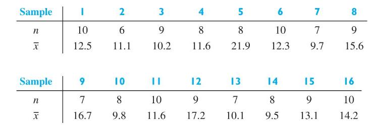
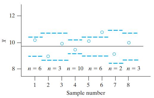
Reverse-current readings (in nanoamperes) are made at the location of a transistor on an integrated circuit. A sample of size 10 is taken every half hour. Since some of the units may prove to be "shorts" or "opens," it is not always possible to obtain 10 readings. The following table shows the
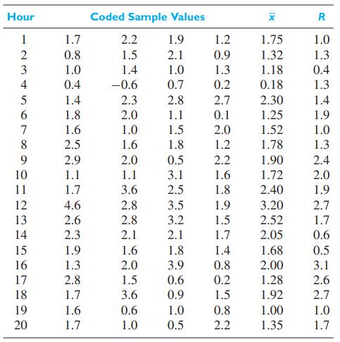
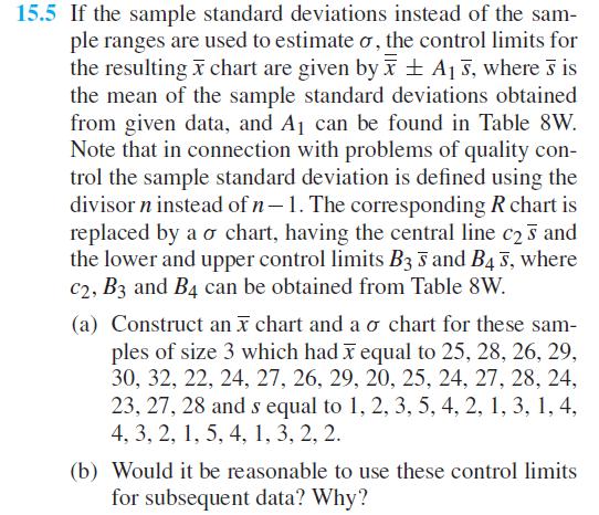
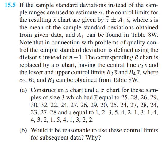
If the sample standard deviations instead of the sample ranges are used to estimate \(\sigma\), the control limits for the resulting \(\bar{x}\) chart are given by \(\overline{\bar{x}} \pm A_{1} \bar{s}\), where \(\bar{s}\) is the mean of the sample standard deviations obtained from given data, and
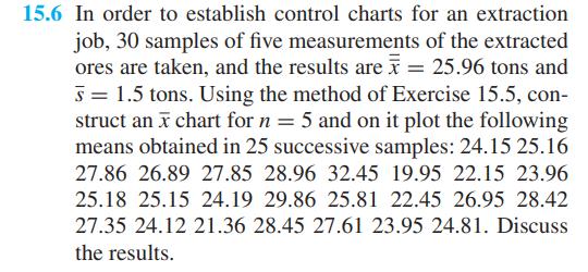
In order to establish control charts for an extraction job, 30 samples of five measurements of the extracted ores are taken, and the results are \(\overline{\bar{x}}=25.96\) tons and \(\bar{s}=1.5\) tons. Using the method of Exercise 15.5, construct an \(\bar{x}\) chart for \(n=5\) and on it plot
Suppose that with the samples of Exercise 15.6, it is desired to establish control also over the variability of the process. Using the method of Exercise 15.5 and the values of \(\overline{\bar{x}}\) and \(\bar{s}\) given in Exercise 15.6, calculate the central line and the central limits for a
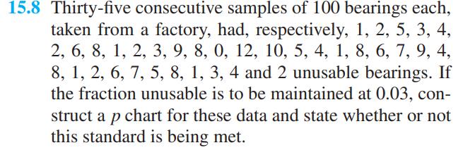
Thirty-five consecutive samples of 100 bearings each, taken from a factory, had, respectively, 1, 2, 5, 3, 4, 2, 6, 8, 1, 2, 3, 9, 8, 0, 12, 10, 5, 4, 1, 8, 6, 7, 9, 4, 8, 1, 2, 6, 7, 5, 8, 1, 3, 4 and 2 unusable bearings. If the fraction unusable is to be maintained at 0.03 , construct a \(p\)
The data of Exercise 15.8 may be looked upon as evidence that the standard of \(3 \%\) unusable bearings is being exceeded.(a) Use the data from Exercise 15.8 to construct new control limits for the fraction unusable.(b) Using the control limits found in part (a), continue the control of the
The specifications for a certain mass-produced valve prescribe a testing procedure according to which each valve can be classified as satisfactory or unsatisfactory (defective). Past experience has shown that the process can perform so that \(\bar{p}=0.03\). Construct a three-sigma control chart
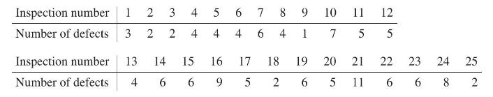
The standard for a process producing tin plate in a continuous strip is 5 defects in the form of pinholes or visual blemishes per 100 feet. Based on the following set of 25 observations, giving the number of defects per 100 feet, can it be concluded that the process is in control to this standard?
A process for the manufacturer of 4-by-8-foot woodgrained panels has performed in the past with an average of 2.7 imperfections per 100 panels. Construct a chart to be used in the inspection of the panels and discuss the control if 25 successive 100-panel lots contained, respectively, 4, 1, 0, 3,
To check the strength of carbon steel for use in chain links, the yield stress of a random sample of 25 pieces was measured, yielding a mean and a standard deviation of 52,800 psi and 4,600 psi, respectively. Establish tolerance limits with \(\alpha=0.05\) and \(P=0.99\), and express in words what
In a study designed to determine the number of turns required for an artillery-shell fuse to arm, 80 fuses, rotated on a turntable, average 45.6 turns with a standard deviation of 5.5 turns. Establish tolerance limits for which one can assert with \(95 \%\) confidence that at least \(99 \%\) of the
In a random sample of 50 electrodes, the mean diameter was \(0.4 \mathrm{~cm}\), and the standard deviation was \(0.005 \mathrm{~cm}\).(a) Between what limits can it be said with \(99 \%\) confidence that at least \(95 \%\) of the diameters of electrodes produced will lie?(b) Find \(99 \%\)
Nonparametric tolerance limits can be based on the extreme values in a random sample of size \(n\) from any continuous population. The following equation relates the quantities \(n, P\), and \(\alpha\), where \(P\) is the minimum proportion of the population contained between the smallest and the
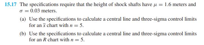
The specifications require that the height of shock shafts have \(\mu=1.6\) meters and \(\sigma=0.03\) meters.(a) Use the specifications to calculate a central line and three-sigma control limits for an \(\bar{x}\) chart with \(n=5\).(b) Use the specifications to calculate a central line and
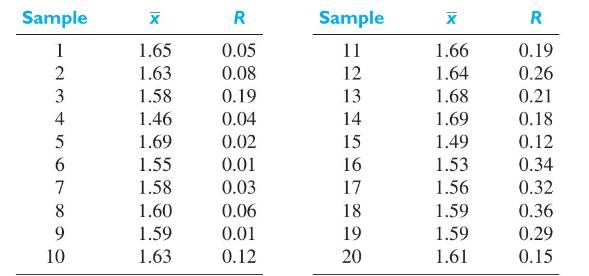
Calculate \(\overline{\bar{x}}\) and \(\bar{R}\) for the data of part (c) of Exercise 15.17 and use these values to construct the central lines and three-sigma control limits for new \(\bar{x}\) and \(R\) charts to be used in the control of the heights of the shock shafts.Data From Exercise 15.17
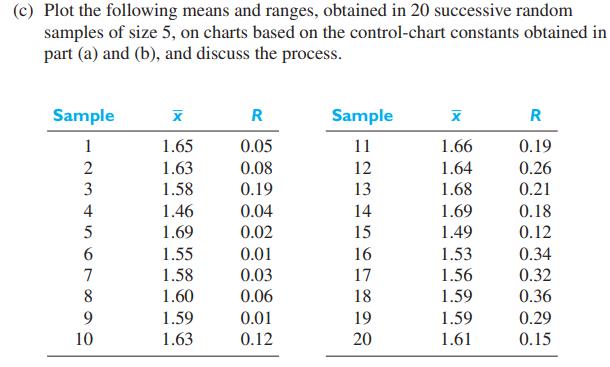
Twenty-five successive samples of 200 propellers, each taken from a production line, contained, respectively, 1, 8, 4, 6, 10, 7, 9, 5, 1, 0, 4, 8, 10, 3, 12, 5, 9, 16, 13, 7, 8, 4, 2, 9 and 2 defectives. If the fraction of defectives is to be maintained at 0.04 , construct a \(p\) chart for these
The data of Exercise 15.19 may be looked upon as evidence that the standard of \(4 \%\) defectives is being exceeded.(a) Use the data of Exercise 15.19 to construct new control limits for the fraction defective.(b) Using the limits found in part (a), continue the control of the process by plotting
A process for the manufacture of film has performed in the past with an average of 0.8 imperfections per 10 linear feet.(a) Construct a chart to be used in the inspection of 10 -foot sections.(b) Discuss the control if 20 successive 10 -foot sections contained, respectively, 1, 0, 0,1, 3, 1, 2, 1,
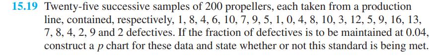
With reference to the aluminum alloy strength data on page 29 , obtain two-sided \(95 \%\) tolerance limits on the proportion \(P=0.90\) of the population of strengths.Data From Page 29 EXAMPLE 7 A density histogram has total area | Compressive strength was measured on 58 specimens of a new
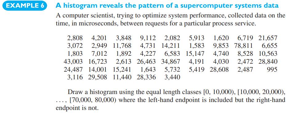
With reference to the interrequest time data on page 29 , obtain \(95 \%\) tolerance limits on the proportion \(P=0.90\) of the population of interrequest times. Take logs, use the normal theory approach, and then transform back to the original scale.Data From Page 29 EXAMPLE 7 A density histogram
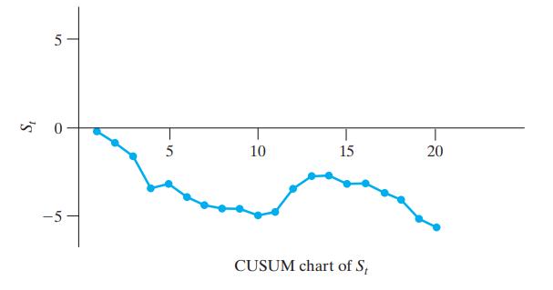
With reference to the discussion on page 492, calculate the CUSUM using 2.25 in place of 2.00 as the centering value. Also make the CUSUM chart.Data From Page 492 5 S -5- 0 5 5 10 15 20 CUSUM chart of S,
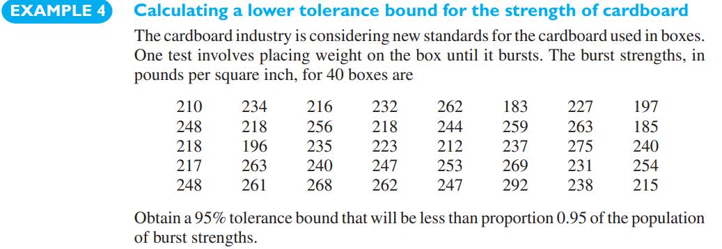
With reference to Example 4.(a) verify the calculation of the tolerance bound \(L\);(b) if the confidence is decreased to \(90 \%\), calculate the new tolerance bound (use \(K=2.010)\)(c) check the cardboard strength data for departures from normality using a normal-score plot.Data From Example 4
Explain, from the perspective of quality improvement programs, why the \(\bar{x}, R\), and fraction defective charts should be used to listen to the process and observe its natural variability, at any stage, rather than for the long-run control of the process.
An experiment is performed to compare the rotational speed of two conveyers, Conveyer \(X\) and Conveyer \(Y\). 30 belts are loaded with an optimal weight, each is put on one of the conveyers, and the speed of the conveyer is measured. Criticize the following aspects of the experiment.(a) To
A certain bon vivant, wishing to ascertain the cause of his frequent hangovers, conducted the following experiment. On the first night, he drank nothing but whiskey and water; on the second night, he drank vodka and water; on the third night, he drank gin and water; and on the fourth night, he
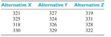
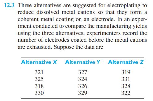
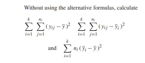
Three alternatives are suggested for electroplating to reduce dissolved metal cations so that they form a coherent metal coating on an electrode. In an experiment conducted to compare the manufacturing yields using the three alternatives, experimenters record the number of electrodes coated before
Using the sum of squares obtained in Exercise 12.3, test at the level of significance \(\alpha=0.01\) whether the differences among the means obtained for the 3 samples are significant.Data From Exercise 12.3 12.3 Three alternatives are suggested for electroplating to reduce dissolved metal cations
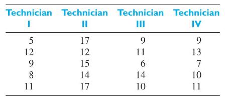
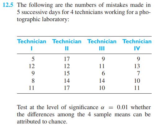
The following are the numbers of mistakes made in 5 successive days for 4 technicians working for a photographic laboratory:Test at the level of significance \(\alpha=0.01\) whether the differences among the 4 sample means can be attributed to chance. Technician Technician Technician Technician I
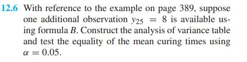
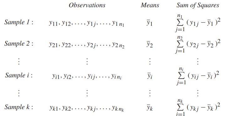
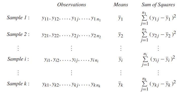
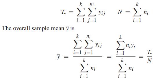
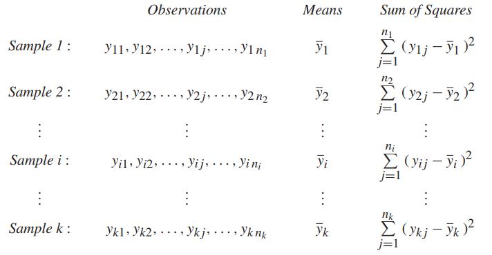
With reference to the example on page 389 , suppose one additional observation \(y_{25}=8\) is available using formula \(B\). Construct the analysis of variance table and test the equality of the mean curing times using \(\alpha=0.05\). Observations Means Sum of Squares Sample 1: Y11 y12 y1jY1n y1
Given the following observations collected according to the one-way analysis of variance design,(a) decompose each observation \(y_{i j}\) as\[y_{i j}=\bar{y}+\left(\bar{y}_{i}-\bar{y}\right)+\left(y_{i j}-\bar{y}_{i}\right)\]and obtain the sum of squares and degrees of freedom for each
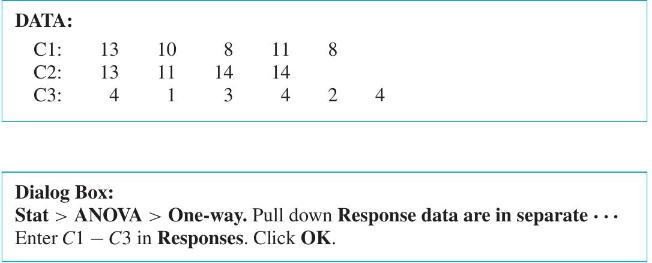
The one-way analysis of variance is conveniently implemented using MINITAB. With reference to the example on page 389 , we first set the observations in columns: DATA: C1: 13 10 C2: 13 11 C3: 4 1 14 83 11 8 14 4 2 4 Dialog Box: Stat > ANOVA > One-way. Pull down Response data are in separate . . .
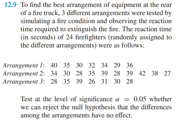
To find the best arrangement of equipment at the rear of a fire truck, 3 different arrangements were tested by simulating a fire condition and observing the reaction time required to extinguish the fire. The reaction time (in seconds) of 24 firefighters (randomly assigned to the different
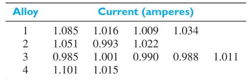
Several different aluminum alloys are under consideration for use in heavy-duty circuit-wiring applications. Among the desired properties is low electrical resistance, and specimens of each wire are tested by applying a fixed voltage to a given length of wire and measuring the current passing
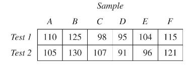
Two tests are made of the compressive strength of each of 6 samples of poured concrete. The force required to crumble each of 12 cylindrical specimens, measured in kilograms, is as follows:Test at the 0.05 level of significance whether these samples differ in compressive strength. Sample A B C D E
Corrosion rates (percent) were measured for 4 different metals that were immersed in a highly corrosive solution:(a) Perform an the analysis of variance and test for differences due to metals using \(\alpha=0.05\).(b) Give the estimates of corrosion rates for each metal.(c) Find 95% confidence
Assume that the standard deviations of the tin-coating weights determined by any one of the 4 laboratories have the common value \(\sigma=0.012\), and that it is desired to be \(95 \%\) confident of detecting a difference in means between any 2 of the laboratories in excess of 0.01 pound per base
Show that if \(\mu_{i}=\mu+\alpha_{i}\) and \(\mu\) is the mean of the \(\mu_{i}\), it follows that\[\sum_{i=1}^{k} n_{i} \alpha_{i}=0\]
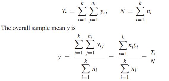
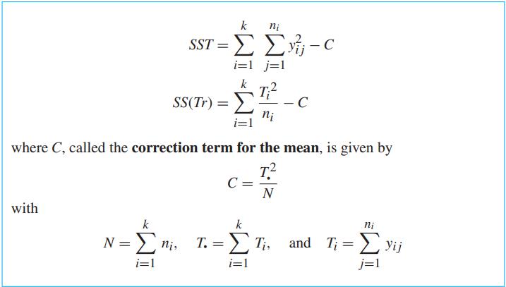
Verify the alternative formulas for computing \(S S T\) and \(S S(T r)\) given on page 399 .Data From Page 399 k ni SST=-C i=1 j=1 k SS(Tr) = ni i=1 where C, called the correction term for the mean, is given by T C N with k k ni N = ni, T. = Ti, and T =yij i=1 i=1 j=1
With reference to Exercise 12.9, determine individual \(95 \%\) confidence intervals for the differences of mean reaction times.Data From Exercise 12.9 12.9 To find the best arrangement of equipment at the rear of a fire truck, 3 different arrangements were tested by simulating a fire condition and
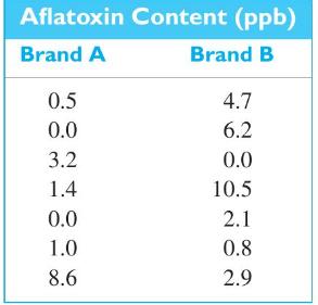
Samples of peanut butter produced by 2 different manufacturers are tested for aflatoxin content, with the following results:(a) Use analysis of variance to test whether the two brands differ in aflatoxin content.(b) Test the same hypothesis using a two sample \(t\) test.(c) We have shown on page
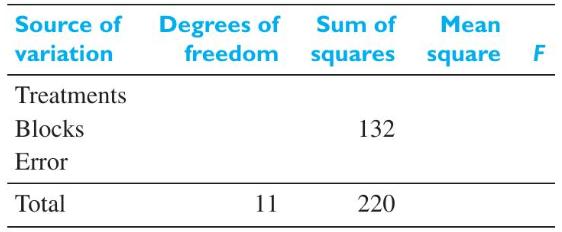
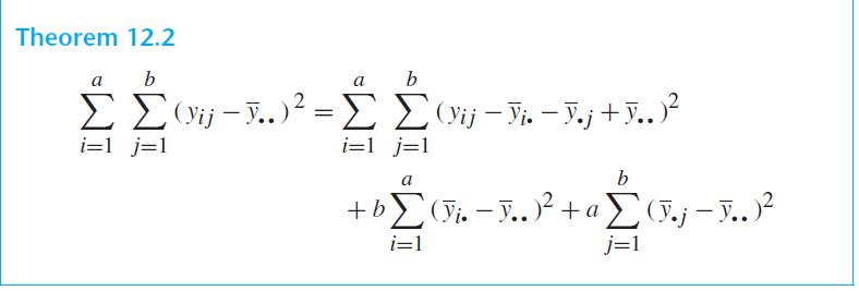
A randomized-block experiment is run with three treatments and four blocks. The three treatment means are \(\bar{y}_{1}=6, \bar{y}_{2 \bullet}=7\), and \(\bar{y}_{3 \bullet}=11\).The total (corrected) sum of squares is\[220=\sum_{i=1}^{3} \sum_{j=1}^{b}\left(y_{i j}-\bar{y}_{\bullet
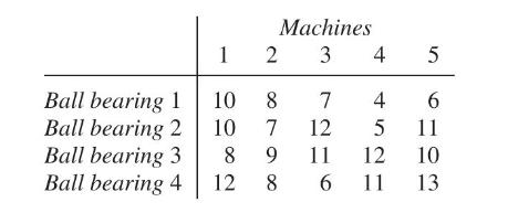
Concerns about the increasing friction between some machine parts prompted an investigation of four different types of ball bearings. Five different machines were available and each type of ball bearing was tried in each machine. Given the observations on temperature, coded by subtracting the
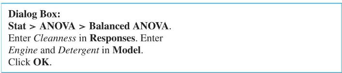
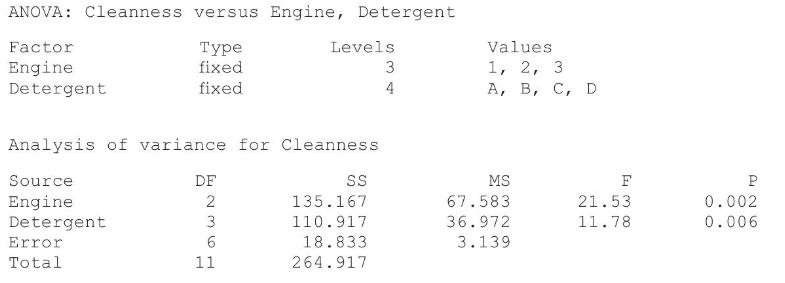
The analysis of variance for a randomized-block design is conveniently implemented using MINITAB. With reference to Example 7, first open C12Ex7.MTW in the MINITAB data bank.Use computer software to re-work Example 6.Data From Example 6 Dialog Box: Stat ANOVA > Balanced ANOVA. Enter Cleanness in
Looking at the days (rows) as blocks, rework Exercise 12.5 by the method of Section 12.3.Data From Exercise 12.5 12.5 The following are the numbers of mistakes made in 5 successive days for 4 technicians working for a pho- tographic laboratory: Technician Technician Technician Technician I II IV 5
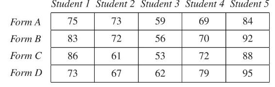
Four different, though supposedly equivalent, forms of a standardized reading achievement test were given to each of 5 students, and the following are the scores which they obtained:Treating students as blocks, perform an analysis of variance to test at the level of significance \(\alpha=\) 0.01
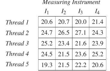
A laboratory technician measures the breaking strength of each of 5 kinds of linen thread by means of 4 different instruments and obtains the following results (in ounces):Looking at the threads as treatments and the instruments as blocks, perform an analysis of variance at the level of
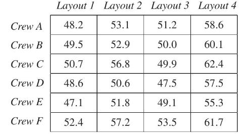
An industrial engineer tests 4 different shop-floor layouts by having each of 6 work crews construct a subassembly and measuring the construction times (minutes) as follows:Test at the 0.01 level of significance whether the 4 floor layouts produce different assembly times and whether some of the
To emphasize the importance of blocking, reanalyze the cleanness data Example 7 as a one-way classification with the 4 detergents being the different treatments.
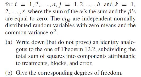
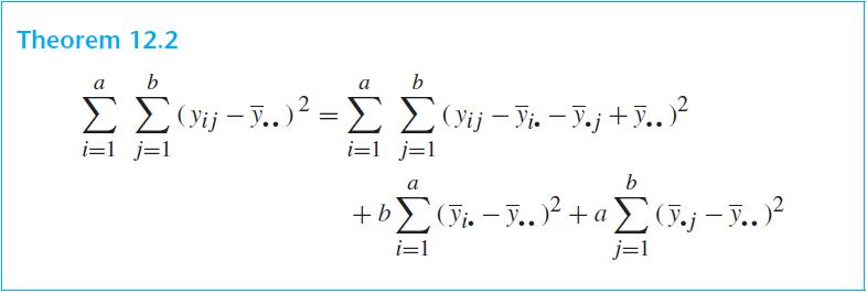
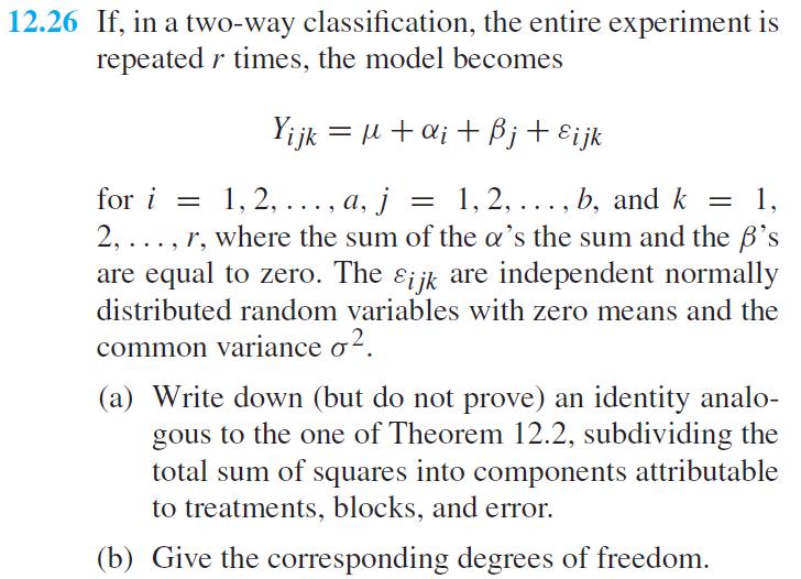
If, in a two-way classification, the entire experiment is repeated \(r\) times, the model becomes\[Y_{i j k}=\mu+\alpha_{i}+\beta_{j}+\varepsilon_{i j k}\]Data From Theorem 12.2 for i = 1, 2,..., a, j = 1, 2, ..., b, and k = 1, 2,..., r, where the sum of the a's the sum and the 's are equal to
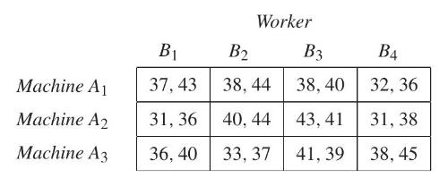
The following are the number of defectives produced by the 4 workers operating, in turn, 3 different machines. In each case, the first figure represents the number of defectives produced on a Friday and the second figure represents the number of defectives produced on the following Monday:Use the
As was pointed out on page 308 , two ways of increasing the size of a two-way classification experiment are(a) to double the number of blocks,(b) to replicate the entire experiment. Discuss and compare the gain in degrees of freedom for the error sum of squares by the two methods.Data From Page 308

Showing 5700 - 5800 of 7136

First
51
52
53
54
55
56
57
58
59
60
61
62
63
64
65
Last

Step by Step Answers

Services

Sitemap
Fun
Definitions
Become Tutor
Used Textbooks
Study Help Categories
Recent Questions
Expert Questions
Campus Wear
Sell Your Books

Company Info

Security
Copyrights
Privacy Policy
Terms & Conditions
SolutionInn Fee
Scholarship
Online Quiz
Give Feedback, Get Rewards

Get In Touch

About Us
Contact Us
Career
Jobs
FAQ
Student Discount
Campus Ambassador

Secure Payment

Download Our App

© 2026 SolutionInn. All Rights Reserved