New Semester
Started
Get
50% OFF
Study Help!
--h --m --s
Claim Now
Question Answers
Textbooks
Find textbooks, questions and answers
Oops, something went wrong!
Change your search query and then try again
S
Books
FREE
Study Help
Expert Questions
Accounting
General Management
Mathematics
Finance
Organizational Behaviour
Law
Physics
Operating System
Management Leadership
Sociology
Programming
Marketing
Database
Computer Network
Economics
Textbooks Solutions
Accounting
Managerial Accounting
Management Leadership
Cost Accounting
Statistics
Business Law
Corporate Finance
Finance
Economics
Auditing
Tutors
Online Tutors
Find a Tutor
Hire a Tutor
Become a Tutor
AI Tutor
AI Study Planner
NEW
Sell Books
Search
Search
Sign In
Register
study help
business
probability and stochastic modeling
Probability And Stochastic Modeling 1st Edition Vladimir I. Rotar - Solutions
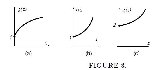
Which functions g(z) in Fig. 3abc look as m.g.f.’s?
Show that if P(X ≥ 3) = 0.2, then the corresponding m.g.f. M(z) ≥ 0.2e3z. What can we say about the distribution of X if M(z) ∼ 0.2e3z as z→∞ ?
Let M(z) be the m.g.f. of a r.v. X. When does there exist at least one number z0 > 0 such that M(z0) < 1 ? Justify your answer.
Let M(z) be the m.g.f. of a r.v. X such that E{X} = 1. Is it true that M(z) ≥ 1 for all z ≥ 0? Answer the same question for the case E{X} = −1.
Let M(z) be the m.g.f. of a r.v. X, E{X} = m, Var{X} = σ2. Write M′(0) and M″(0).
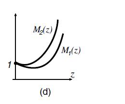
Compare the means and variances of the r.v.’s whose m.g.f.’s are graphed in Fig. 3d.
(a) Can the function 1+z4 be the m.g.f. of a r.v.?(b) In general, show that if g(z) = 1+ε(z)z2, where ε(z) ≠ 0 for z ≠ 0, and ε(z) → 0, as z→0, then g(z) cannot be a m.g.f.
Prove that the sum of independent Poisson r.v.’s is Poisson by the method of m.g.f.’s.
We come back to Section 2.2. Show that the function fS(x) = e−x/2 −e−x for x ≥ 0 and = 0 otherwise is a probability density; that is, it is non-negative and the total integral is one.
Using the method of m.g.f.’s, find the density of the sum of two independent exponential r.v.’s with means 2 and 3, respectively.
If Sn = X1 +...+Xn, where the X’s are i.i.d., then as we know, MSn (z) = (MX (z))n, where MX (z) is the m.g.f. of Xi. Show that Proposition 2 includes this case.
The number of customers of a company for a randomly chosen day is a Poisson r.v. with parameter λ = 50. The amount spent by each customer is an exponential r.v. with a mean of m = 100. All the r.v.’s involved are independent. Write the m.g.f. of the total daily income.
Assume that, in an area, the number of traffic accidents on a randomly chosen day is a Poisson r.v. with λ = 300, and the probability that a separate accident causes serious injuries is p = 0.07. The outcomes of different accidents are independent. Find the probability that the number of accidents
Assume that, in an area, the number of traffic accidents on a randomly chosen day is a Poisson r.v. with parameter λ1, and the number of injuries a particular accident causes is a Poisson r.v. with parameter λ2. Write the m.g.f. of the total number of injuries. The corresponding distribution is
The number of customers of a company during a randomly chosen day is a r.v. K for which P(K = k) = 1/3(2/3)k, k = 0,1, .... The amount spent by a particular customer is an exponential r.v. with a mean of $1,000. All the r.v.’s involved are independent. Find the probability that the daily income
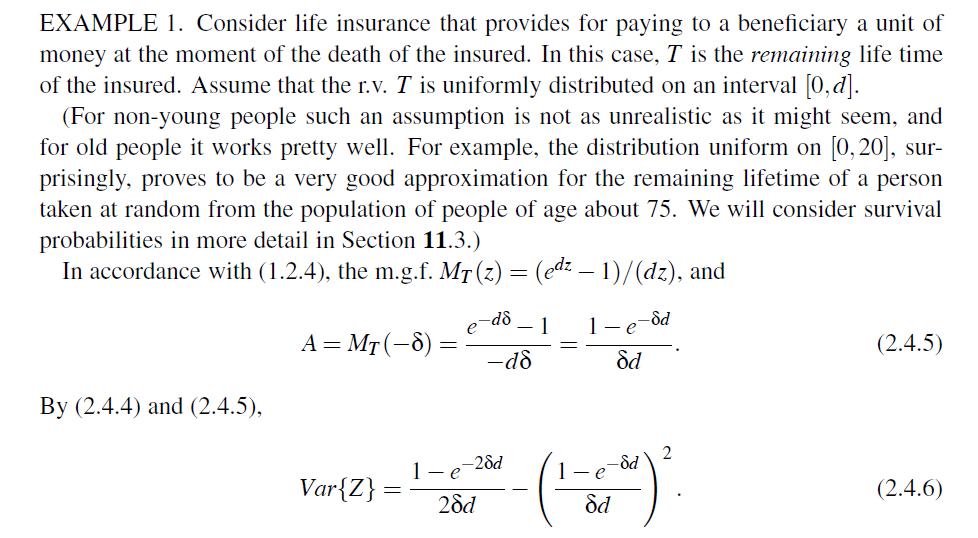
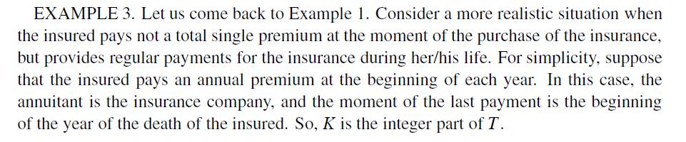
Solve the problems of Examples 2.4-1,3 (that is, find the quantities A, a, and π) for the case when the remaining lifetime T is exponential with parameter μ (we are using the symbol a for other purposes). For simplicity and to make formulas nicer, suppose, that the premium payment is provided
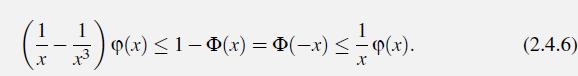
Write a bound of the type (3.1.2) for the standard normal distribution and compare it with the bound (6.2.4.6). Which is better? Do you find the difference significant?
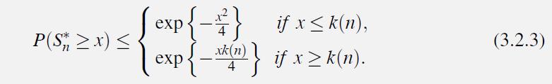
John and Mike play a game consisting in tossing a coin. If the coin comes up heads John pays to Mike $1. Otherwise, it is Mike who pays $1. Let Sn is Mike’s gain (which may be negative) after n tosses. Using (3.2.3), write a bound for P(Sn > x) and x > 0.
In a poll concerning future elections, 55% of 1,500 respondents said that they would vote for Candidate A. To what degree can we expect that A will win?
On Sundays, Michael sells the Sunday issue of a local newspaper. The mean time between consecutive buyers is 3 min., and the corresponding standard deviation is 1.5 min. Estimate the time period that will be sufficient to sell 60 copies on 80% of Sundays on the average.
A surveyor is measuring the distance between two remote objects with use of geodesic instruments from 25 different positions. The errors of different measurements are independent r.v.’s with zero mean and a standard deviation of 0.1 length units. Estimate the probability that the average of the
Let Sn = X1 +...+Xn, where X’s are independent and uniform on [0,1]. Consider S∗n = (Sn − n/2)/√n/12. Explain why it makes sense to consider this r.v. Using software, for n = 5, 10, 20, simulate a number of values (say, 1000) of S∗n, and make histograms (see Section 7.5). Compare these
A regular die is rolled n times. Let Sn be the total sum of the numbers showed up. Say without calculations what Sn is equal to on the average. For a > 0, let a+n = 3.5n+a√n, a−n = 3.5n − a√n, and qn(a) = P(a−n ≤ Sn ≤ a+n). (a) Show that qn(a) → q(a) as n → ∞, where q(a) is a
Let X1,X2, ... be a sequence of independent r.v.’s uniformly distributed on the interval [0,2], and let Sn = X1 + ... + Xn.(a) Find E{Sn} and Var{Sn}.(b) Using the Central Limit Theorem, estimate P(n − √n ≤ Sn ≤ n + √n).(c) Write down a formula for the limit ofProceeding from the
Let X1,X2, ... be a sequence of independent exponential r.v.’s with E{Xi} = 2, and let Sn = X1+...+Xn. Find limn→∞ P(Sn ≤ 2n+ √n).
An energy company provides services for a town of n=10,000 households. For a household, the size of monthly energy consumption is exponentially distributed with a mean of 800 kwh, and does not depend on the consumption of other households. The company has specified a consumption baseline d which is
Show that the negative binomial distribution with parameters (p, ν) may be well approximated by a normal distribution for large ν. State the CLT for this case.
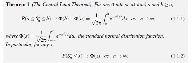
Let Y be a standard normal r.v., and for a set B in the real line, let Φ(B) = P(Y ∈ B). From Theorem 1, we know that P(S∗n ∈ B) → Φ(B) as n → ∞ if B is an interval. Is the same true for any B? (Advice: Consider Xj = ±1 with equal probabilities, and realize that in this case S∗n = 1
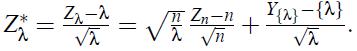
Show that the distribution of Zλ may be approximated by a normal distribution for any large, not necessary integer, λ. (Advice: First, λ = [λ]+{λ}, where [λ] is the integer part of λ, and {λ}=λ−[λ], the fractional part of λ. Accordingly, with n = [λ], we may write Zλ = Zn + Y{λ},
What would the probability that the company will not suffer a loss have been equal to if the premium had been equal to the mean payment?
Consider the probability that the company will not suffer a loss. Using the particular data from this example, for a portfolio of n = 1000 independent policies, find a single premium (that is, the premium paid at the moment of policy issue) for which this probability is not smaller than 0.9. (The
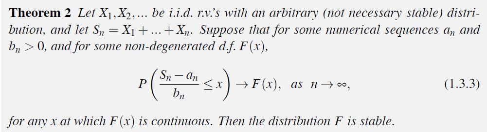
Proceeding from Theorems 2 and 3, explain why the Cauchy distribution (which is stable) cannot be a limiting distribution for the normalized sum of i.i.d. r.v.’s with a finite variance.
Under which conditions is (2.1.2) true if the X’s are normal?
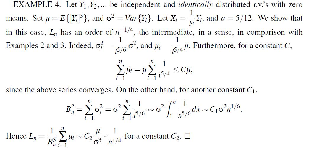
Consider a generalization of Example 2.1-4 for an arbitrary parameter a. For which a does the CLT hold? Consider the order of the Lyapunov fraction Ln (and hence, the rate of convergence in the CLT) for different a’s.
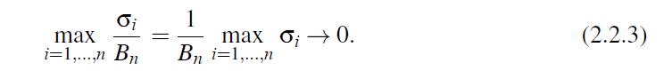
Show that if (2.2.3) holds, then all terms Xi/Bn are asymptotically negligible; more precisely, that
Lindeberg’s condition (2.2.2) requires Λ(ε)→0 for any ε > 0. Can it be true for ε = 0? To what, as a matter of fact, is Λ(0) equal?
Mark each statement below “true” or “false”. Justify your answers.(a) Cov{X1,X2} =Cov{X2,X1}.(b) If two r.v.’s are independent, then they are uncorrelated.(c) If two r.v.’s are correlated, then they are dependent.(d) If two r.v.’s are uncorrelated, then they are independent.(e) A
(a) Show that for Cov{X1,X2} = E{X1X2}, it suffices that either X1 or X2 has zero mean.(b) Show that Cov{X +Y,Z} =Cov{X,Z}+Cov{Y,Z}.
(a) What is Cov{X,−X}, Cov{−X,−X})?(b) Let c =Cov{X1,X2}. Write Cov{2X1,3X2}, Cov{−2X1,3X2}, Cov{−2X1,−3X2}.(c) Let ρ = Corr{X1,X2}. Write Corr{X1,−X2}, Corr({X1,10−X2}, Corr{2X1,3X2}, Corr{−2X1,3X2}, Corr{−2X1,−3X2}. In general, how will Corr{X1,X2} change if we multiply X1
Let a r.vec. (X,Y) be uniformly distributed on the disk {(x,y) : x2 + y2 ≤ 4}. Find the covariance. Are X,Y independent? Do the same for the uniform distribution on {(x,y) :x2 +x+y2−3y≤ 20}.
Does it follow from the Cauchy-Schwartz inequality (Proposition 1) that for any r.v.’s ξ and η with finite second moments, (E{|ξη|})2 ≤ E{ξ2}E{η2}? Which inequality is stronger: this or (1.2.1)?
Two dice are rolled. Let X and Y be the respective numbers on the first and the second die, and Z =Y −X.(a) Do you expect negative or positive correlation between X and Z?(b) Find Corr{X,Z}. (Advice: Use the particular information about the distribution of (X,Y) at the very end, if
Let r.v.’s X and Y be independent, Z1 = X +Y, Z2 = X −Y. When are the r.v.’s Z1 and Z2 uncorrelated? Would it mean that they are independent? Let, say, (X,Y) be uniformly distributed on the square {(x,y) : |x| ≤ 1, |y| ≤ 1}. If we know X +Y, does it give an additional information about
Let r.v.’s X and Y be independent, Z = X +Y. Find Corr{X,Z} as a function of the ratio k =Var{Y}/Var{X}. Comment on the fact that this function is monotone.
Two balls, one at a time, are drawn without replacement from a box containing r red and b black balls.(a) For i = 1, 2, let Xi = 1 if the ith ball is red, and Xi = 0 otherwise. Do you expect negative or positive correlation between X1 and X2? Compute Corr{X1,X2}.(b) Let Y1 and Y2 be the numbers
Suppose n balls are distributed at random into k boxes. Let Xi = 1 if box i is non-empty, and Xi =0 otherwise. Argue that Corr{Xi,Xj}=Corr{X1,X2} for all i = j and findCorr{X1,X2}.
Let a r.vec. (X,Y) have the joint density f(x,y)= 3/8 (x+y)2 for |x|≤ 1, |y|≤1, and f (x,y)=0 otherwise. Do you expect the r.v.’s to be dependent? Find Corr{X,Y}. (Use of software is recommended.)
You are working with r.v.’s X1,X2,X3, ... , and you are interested only in their variances and correlations. Can you switch to the centered r.v.’s and deal only with them?
Prove (1.1.11).
John invests one unit of money in two business projects; an amount of α goes to the first, and 1−α goes to the second. For i = 1, 2, let Xi be the (random) return (per $1) of project i. It is known that the means of X1 and X2 are the same. The variances σ2i = Var{Xi} and ρ = Corr{X1,X2} ≠
Let X1,X2,X3,X4 be independent r.v.’s with variances 1,2,3,4, respectively. Do you need to know the mean values of X1,X2,X3,X4 in order to compute the correlations of(a) X1 + X2 and X2+X4;(b) X1+X2 and X3+X4? Compute the correlations mentioned.
(a) Let X be uniform on [−1,1], andY = X3. Find ρ =Corr{X,Y} and explain why ρ ≠ 1 while the association (or dependence) is perfect and positive.(b) Solve the same problem for Y = X2k+1, where k is a positive integer.
Represent the “beta of security” terms of the correlation coefficient ρ =Corr{X,Y}.
In a country, the mean weight of adult females is 110 lb, and the mean height is 155 cm. The respective standard deviations are 15 and 12. Ms. K weighs 114 lb, and her height is 159 cm.The same figures forMs. S are 105 lb and 149 cm. Estimate the correlation proceeding from a linear regression
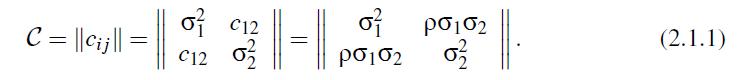
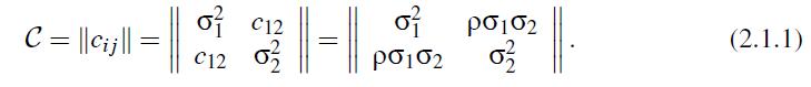
For which ρ does there exist the inverse of C in (2.1.1)?
Given the covariance matrix C of a r.vec. (X1, ...,Xk), how to compute the variance of the sum X1+...+Xk?
Let X be a r.vec., E{X} = 0, and Y = Q X, where Q is a non-random orthogonal matrix. Using a probability theory argument, prove that the covariance matrices CY and CX have the same traces (the sums of the diagonal entries).
Let (X1, ...,Xk) be a r.vec. with a covariance matrix C. Under which condition on C does there exist a linear combination t1X1+...+tkXk with zero variance and with not all t’s equal zero?(Say, you have estimated the covariance matrix of the returns of a collection of securities in a financial
Let X = (X1, ...,Xk) be a random vector with a covariance matrix C, and t = (t1, ..., tk) and ˜t= (˜t1, ..., ˜tk) be two non-random vectors. Consider two linear combinations: 〈X, t〉 and 〈X,˜t〉. Generalizing (2.1.4), prove that Cov{〈X, t〉, 〈X,˜t〉} = 〈Ct,˜t〉. Can we switch t
Regarding relation (2.2.2), show thatExplain why a squared loading coefficient may be viewed as the percentage of the factor variance “contributed” to the variance of the component.
This exercise concerns the theory of Section 2.3. Suppose that a financial market consists of two securities with expected returns of 6% and 8%, and standard deviations of 1% and 2%, respectively. Let the correlation ρ = 0.3.(a) Consider two portfolios: x = (1/2, 1/2), and y = (1/3, 2/3). Let Rx
Let f (x1,x2) be the density of a r.vec X = (X1,X2). We call a curve in a (x1,x2)-plane a level curve if it is determined by an equation f (x1,x2) = c, where c is a constant. Argue that all points in this curve are equally likely to be values of X. Show that for a bivariate normal distribution,
Let X and Y be independent standard normal r.v.’s, Z1 = X +Y, Z2 = X −Y. Are Z1 and Z2 independent?
Let a r.vec (X1,X2) is normal with zero means and covariance matrix (2.1.1). Write the density of X1+X2.
Let X = (X1, X2) be a two-dimensional normal random vector; E{X1} = 1, E{X21} = 5, E{X2} = 2, E{X21} = 13, E{X1X2} = −2.(a) Write the density of the centered vector Y = X−m, where the vector m = (1,2). Write the density of X.(b) For t = (3,−4), (i) write the expectation, the variance and
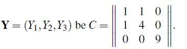
Let the covariance matrix of a normal r.vec.Explain without any calculations why Y3 does not depend on the r.vec. (Y1,Y2). Assuming E{Y} = 0, write the density of Y.
Let us present a two-dimensional standard normal r.vec. X in the polar coordinates as (R, Θ), where R is the length of X and Θ is the angle between X and the first axis.(a) Are the r.v.’s R, Θ independent? What are the marginal distributions?(b) Would you expect the independence of R and Θ
Let B be a rotation matrix, X be a standard normal r.vec., and Y = BX. What is the distribution of |Y|2?
In the framework of Section 3.2, find the density of the r.v. χk = |X|.
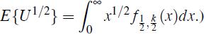
Show that E{χk} = √2Γ((k + 1)/2)/Γ(k/2). (Advice: A simple way is to consider a r.v. U having the χ2k -distribution; that is, the Γ-distribution with parameters (1/2 , k/2 ), and write the integral for
Continue the calculations. (Advice: You may choose a slightly heuristic approach using the representation ξk = 1/√k Yk, where Yk = 1/√k Σki=1(X2i−1), and Xi’s are standard normal. For large k, by the CLT, Yk is asymptotically normal, which gives a clue how to estimate the moments of ξk.)
John throws a dart at a circular target with a radius of r. Suppose that with respect to a system of coordinates with the origin at the center of the target, the point where the dart lands may be represented as a bivariate normal vector Y = r/4 X, where X is a standard normal vector. (In
In the case you solved Exercise 36, find the mean speed of a molecule. (Advice: Use the fact that Γ(t +1) = tΓ(t).)Exercise 36Show that E{χk} = √2Γ((k + 1)/2)/Γ(k/2). (Advice: A simple way is to consider a r.v. U having the χ2k -distribution; that is, the Γ-distribution with parameters
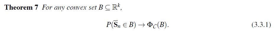
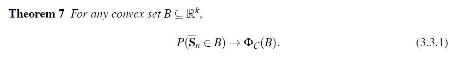
Restate Theorem 7 for the one dimensional case. How does this restatement differ from Theorem 1 from Chapter 9? Show that both assertions are equivalent.
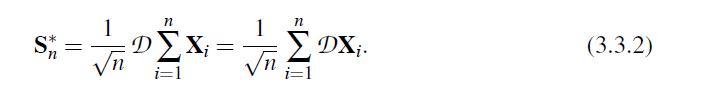
What is the matrix D in (3.3.2) if the matrix C in Section 3.3 is diagonal?
Suppose that the coordinates of a r.vec. X = (X1, ...,Xk) are independent. Present the m.g.f MX(z) in terms of the m.g.f.’s of the coordinates. Is MX(z) uniquely determined by the m.g.f.’s of the coordinates in the general case? (Advice: As an example, we may consider the normal case, and
In Section 3.3, let k = 2, and separate terms Xi = (Xi1,Xi2), where Xi1,Xi2 are independent and have the standard exponential distribution. Let the vector e= (1,1). For large n, estimate P(|Sn −n · e| ≤ √n).
Is (3.3.1) true for the sets depicted? Theorem 7 is stated for convex sets, but it does not mean that (3.3.1) cannot be true for a non-convex set.
For a husband and wife, the future lifetimes are independent continuous r.v.’s X1 and X2. Suppose the tail functions F̅1(x) = P(X1 > x) and F̅2(x) = P(X2 > x) are given. Find the probabilities that(a) Both will survive n years;(b) Exactly one will survive n years;(c) No one will survive n
(a) In a closed auction, the buyers submit sealed bids so that no bidder knows the bids of the others. The highest bid wins. Suppose that the bids are independent r.v.’s uniformly distributed on [a,a+d]. For the case of n bidders, find the distribution and expectation of the price for which the
Each day, John is jogging the same route. The times it takes are i.i.d. r.v.’s assuming values between 30 and 31 minutes. Find the distribution of the best result in a week and its expected value in the case where for each separate day(a) The distribution is uniform on [30,31]; (b) The
Let X1,X2,X3, ... be independent exponential r.v.’s, and let E{Xi} = 2i. Find the distribution of min{X1,X2, ...} or, more precisely, the limiting distribution of
Comment on the behavior of the expectations for large n. If you pick (or simulate) 100 independent numbers from [0,1], to what will the largest and the smallest number be close? The reader who chose Route 2, may also come back to this question after she/he reads Section 2.1.
The time to failure for each of particular standard electronic devices has the density f (x) = 64/x5 for x ≥ 2. Show that the corresponding r.v.’s are larger than 2 with probability one. Let Tn be the time to failure for a series of n such devices. Guess to what E{Tn} should converge as
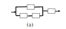
Consider the system with the configuration presented in Fig. 10a and suppose that all components work independently. Let the time to failure for a separate component have a d.f. F(x).Find the d.f. of the time to failure for the whole system. Will your answer change if the signal moves in the
A system consists of two components, and for the system to work, at least one component should work. The times to failure for the components are independent and exponential with a mean of one unit of time. For which time period is the probability that the system will not fail during this period is
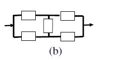
Consider the configurations in Fig. 10b, suppose that the lifetimes of the separate components are independent, denote by G(x) the d.f. of the lifetime of the “middle” component, and suppose that the other components have the same lifetime d.f. F(x). Find the d.f. of the system lifetime.
Consider i.i.d. r.v.’s X1,X2, ... assuming a finite number of values x1 2 m. (a) Describe the behavior of the r.v.’sandheuristically.(b) Provide a rigorous explanation. How “fast” do the distributions of approach their limits (if any)?(c) Describe the cases where we cannot expect a
Prove (2.1.2).
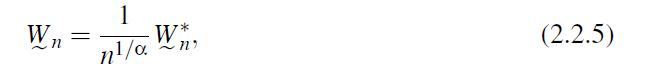
What is α and the distribution of W̰*nin the case (2.2.5) if the X’s are exponential?
Write the limiting distribution and representation (2.2.5) for the X’s having(a) The density f(x) = 2x for x ∈ [0,1];(b) The density f(x) = 1/2(2−x) for x ∈ [0,2].
Write the limiting distribution and representation (2.2.6) for the X’s having the density f(x)= 2(x−1) for x ∈ [1,2]. Compare with Exercise 13a.Exercise 13aWrite the limiting distribution and representation (2.2.5) for the X’s having(a) The density f(x) = 2x for x ∈ [0,1];
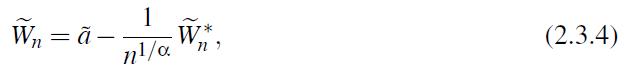
Write the limiting distribution and representation (2.3.4) for the following situations:(a) The density of the X’s is f (x)=2(x−1) for x ∈ [1,2];(b) The density of the X’s is f (x)=3(2−x)2 for x ∈ [1,2];(c) The r.v. Xi = −ξi, i = 1,2, ..., where ξi are independent standard
Show that if in the normalization procedure (2.2.2), we multiply W̰n by (cn)1/α, then the limiting distribution will be the Weibull distribution Q1α(x) = 1−exp{−xα}.
Regarding Propositions 1 and 2, does the increase of the parameter α lead to the faster or slower rate of convergence to the limit? Give a rigorous answer and a heuristic commonsense interpretation.
Prove that the expected value of the estimate W̃n, that is, E{W̃n} = n+1 θ. Such an estimate is called biased: its expected value is not equal to the parameter we are estimating. By what should we multiply W̃n for the new estimate, Ṽn, to have the following two properties: first, Ṽn is
Let X1, ...,Xn have Weibull’s distributions Qc1α, ...,Qcnα, respectively. Show that the min{X1, ...,Xn} has the distributionQcα with c = c1+...+cn. That is, the Weibull distribution is stable with respect to minimization. Connect this fact with the result of Proposition 5.
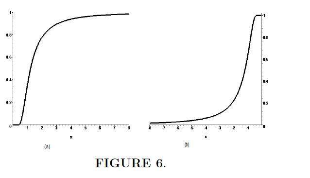
Make sure that you understand why the graphs of and indeed look as they are depicted in Fig. 6.
Write the limiting distribution and representation (2.4.8) for the X’s having the density f(x)= 64/x5 for x ≥ 2.
Write the limiting distribution, representation (2.4.8) and a similar representation for for Xi’s having the Cauchy distribution (that has the density f (x) = 1/(π(1+x2)).
Showing 6400 - 6500
of 6914
First
56
57
58
59
60
61
62
63
64
65
66
67
68
69
70
Step by Step Answers