New Semester Started Get 50% OFF Study Help! --h --m --s Claim Now

Question Answers

Textbooks

Find textbooks, questions and answers

Oops, something went wrong!

Change your search query and then try again

Result Not Found

Books FREE
Study Help
Tutors
AI Study Planner NEW
Sell Books

Search
Sign In
Register

study help
business
probability and stochastic modeling

Probability And Stochastic Modeling 1st Edition Vladimir I. Rotar - Solutions

Let wt be Brownian motion.(a) Are w1 and w5 independent r.v.’s?(b) Answer the same question for w1 and w(1,5].(c) Find P(w1+w5 < 4).
Let wt1 and wt2 be independent Brownian motions. Find σ for which the process wt1 +2wt2 has the same distribution as σwt1.
Consider the process xt = σ1wt1 +σ2wt2, where σ1, σ2 are numbers. Let σ2 = σ21 +σ22. Show that the process xt/σis a standard Brownian motion, and hence xt may be represented as σwt, where wt is a standard Brownian motion. Next, consider the case σ1 = −1, σ2 = 0. Explain why the fact
A physical process evolves as wt. You decided to measure time in different units setting t = as, where a is a fixed scale parameter and s is time measured in the new units. Argue that you cannot model the original process by ws. Find c for which the process cws would be an adequate model for the
Assume that in the situation, you decided to sell the stock not when the price increases by 10%, but when it drops by 10%. Will the answer change? If yes, find it. If no, justify the answer.
The prices for two stocks evolve as the processes St1 =10exp{σ1wt1} and St2 =11exp{σ2wt2}, where wt1 and wt2 are independent Brownian motions, σ1 = 0.1, and σ2 = 0.2. What are the initial prices for the stocks? Find the probability that during a year the price St1 will meet the price St2.
Find Corr{wt ,ws} and show that it vanishes as t →∞ for any fixed s.
Show that ∼wt and |wt| have the same distribution.
(a) Compute the probability density of the r.v. τa from Section 1.1.3. Show that E{τa}=∞.(b) Proceeding from the invariance principle, connect heuristically this fact with what we obtained in Example 15.2.2-2: for the symmetric random walk, the mean time of reaching a level a equals infinity.
Prove that E{∼wt} = √2t/π. Show that to obtain this answer, it suffices to consider the case t = 1. Is the expected value of the maximum value of Brownian motion on the interval [0,2] twice as large as that on the interval [0,1]?
For any non-random interval Δ, the r.v. wΔ is normal. Is it true if Δ is random? Give an example. Is the r.v. w(τa, t] normal? Look also at the proof of (1.1.6).
Customers are calling to a company, and each customer is equally likely to be a man or a woman. Using the Brownian motion approximation, estimate the probability that during the first n = 100 calls, the difference between the numbers of men and women will not exceed a = 10. (Advice: When applying
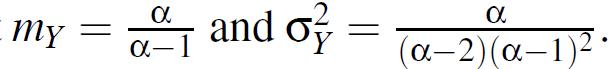
Find E{Yt} and Var{Yt} for the geometric Brownian motion Yt defined in Section 1.2. (Advice: Use the formula for the m.g.f. of the normal distribution.)
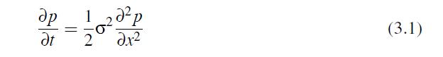
Suppose that the “chaotic”motion of a particle along a line is depicted by a Markov process Yt with continuous trajectories. Let p(y|x, t) be the density of Yt under the initial-time condition Y0 = x. A. Einstein has shown that the function p(y|x, t) should satisfy the equationwhich is called
Show that any process ξt with independent increments such that E{ξΔ} = 0 for any interval Δ, is a martingale. Consider, as an example, wt. Explain why the assertion of this exercise is formally more general than the assertion of Example 2.1-1 (though it is very close).
Let Nt be a non-homogeneous Poisson process. Is Nt a martingale? Is the process Xt = Nt −E{Nt} a martingale (with respect towt )?
Show that any process Xt such that E{X(t,t+δ] |Xt} = 0 for any t and δ ≥ 0 is a martingale.
Let Yt =Cte4wt . What should the constant Ct be for Yt to be a martingale?
Let a stock price process St be a geometric Brownian motion with an annual volatility of σ = 0.1, and an expected annual return of m = 0.15 per annum. Let S0 = 100.(a) Write a basic differential equation for St and a solution to this equation.(b) Find the probability that at time T = 6 months,
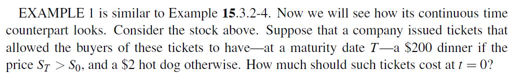
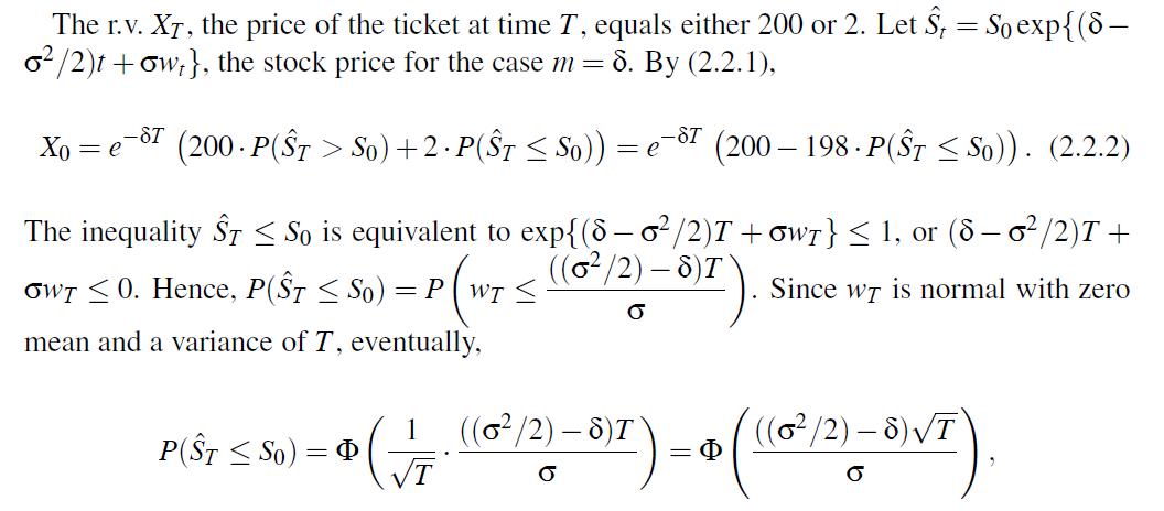
Make sure that the answer in Example 2.2-1 becomes much simpler if δ = 0.
This exercise concerns some properties of the Black-Scholes formulas (2.2.3) and (2.2.4).(a) Consider a call option. If T is very small, the option will be ready to be exercised practically immediately, and hence its price should be close to (S0 −K)+. Show that, indeed, the price in (2.2.3)
Consider the stock described in Exercise 20 and assume the risk-free rate δ = 0.05.(a) Find the prices for a put and call option with an exercise price of K = $100 and maturity time T = 6 months. Show why the general formula becomes simpler in this case.(b) Richard has an $100 bet with John that
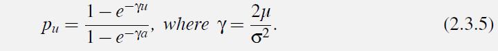
Find the limit of (2.3.5) as μ → 0 and σ fixed. Interpret the answer.
Find the probability that the Wiener process wt will ever hits the line c+bt where c and b are positive numbers.
A capital growth process is well approximated by the Brownian motion with drift Xt = u+ μt +σdwt from Section 2.3.2. The ruin probability for a certain choice of parameters occurs to be 1/16. How will this probability change if(a) The parameter σ is doubled;(b) The process Xt is multiplied by
The level of a water reservoir changes, in appropriate units, accordingly to the process Xt = 1+2t+3wt, where wt is a standard Brownian motion. (Certainly, Xt may be negative, so this is just an approximation.) Find the probability that the reservoir(a) Will never be empty, (b) Will not be empty
You decided to sell the stock not when the price increases by 10% but when it decreases by 10%. Will the answer change? If yes, find it. If no, justify the answer. Is the selling time proper (non-defective) in this case? Find the probabilities that the price will never drop by 10%, and will not
The prices for two stocks change as the processes St1 = 10exp{μ1t + σ1wt1} and St2 = 11exp{μ2t+σ2wt2}, where wt1 and wt2 are independent Brownian motions, μ1 = 0.15, μ2 = 0.11, σ1 = 0.15, and σ2 = 0.1. What are the initial prices for the stocks? Find the probability that during a year the
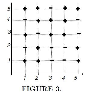
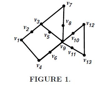
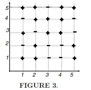
In Example 1.1-1, comment on how (1.1.9) would look for the lattice in Fig. 3.
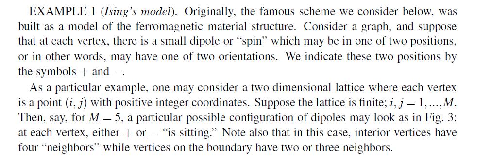
For the scheme,(a) Find the dependency neighborhood of the vertex v6 in Fig. 1;(b) Describe dependency neighborhoods for the lattice in Fig. 3 (certainly, ignoring pluses and minuses there).
Regarding the point process from Section 1.3, is μ(A) a counting measure?
For a point Poisson process NA, find Corr{NA,NB}.
(a) Realize that the integral in (1.3.3) may be computed with use of a table for the standard normal distribution;(b) Model the case where the intensity of fires is growing proportionally to the distance from the center, and find P(Y > r).
Suppose n points are selected at random and independently from a unit cube. Let NA be the number of points fallen in a region A in the cube.(a) Does this point process satisfy the complete randomness condition (1.3.1)?(b) Find the intensity μ(A), and the probability that all points will fall in
Suppose that in the region within ten miles from a hospital, the locations of emergency calls during a particular day are distributed accordingly to a Poisson point process. The region consists of two subregionswith equal areas. In the first, the intensity equals 0.03 per sq. mile, in the second it
State the CLT for the scheme in the case where ξ’s are uniform(a) On [−1,1];(b) On [0,1].
Consider a two-dimensional lattice with vertices v = (i, j); i, j = 1,2, .... To each vertex v, we assign a r.v. ξv and assume ξ’s to be i.i.d. A neighborhood Nv consists of the nearest vertices. Let Xv = ξv · Πu∈Nv ξu (the product of the r.v.’s in the neighborhood). State the CLT for
Let Y,Y1,Y2, ... be i.i.d. r.v.’s, E{Y} = 0, Var{Y} = 1. Let the random vector (X1n, ...,Xnn) = (Y1, ...,Yn) with probability 1−1, and (X1n, ...,Xnn) = (Y, ...,Y) with probability 1. Let Sn = X1n+...+Xnn. Show thatwhile Var{Sn} = 2n−1 ∼ 2n, which says that the standard deviation of the sum
Prove that if Λ has the Γ-distribution with parameters (a, ν), then X’s are negative binomial with parameters (p, ν), where
State the LLN for the scheme. Interpret your result.
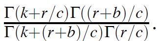
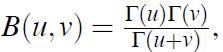
Consider the Polya urn model.(a) Show that the density of Θ is indeed the Beta-density from (4.2.4). In particular, make sure that E{Θ} indeed equals r/b+r. (Advice: Proceeding from the formula Γ(t +1) = tΓ(t), show that the r.-h.s. of (4.2.3) equalsUsing the formulafind the moments of the
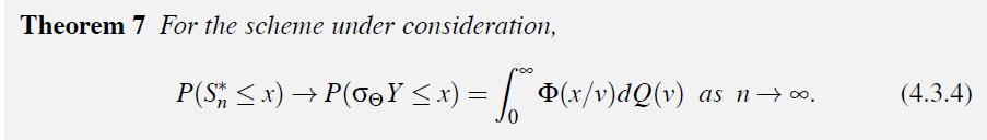
Is the limiting distribution in Theorem 7 always symmetric?
This exercise concerns the VaR criterion with a parameter γ. R.v.’s X below—with or without indices—correspond to an income.(a) Let a r.v. X1 take on values 0,1,2,3 with probabilities 0.1, 0.3, 0.4, 0.2, respectively, and a r.v. X2 take on the same values with probabilities 0.1, 0.4, 0.2,
For the case of the TailVaR criterion, solve(a) Exercise 1a;(b) Exercise 1d.Exercise 1:This exercise concerns the VaR criterion with a parameter γ. R.v.’s X below—with or without indices—correspond to an income.(a) Let a r.v. X1 take on values 0,1,2,3 with probabilities 0.1, 0.3, 0.4,
Let r.v.’s X1, ...,X10 be independent exponential r.v.’s with unit means. Suppose that Yi = 1.1 · Xi for i = 1, ..., 10, represent the returns for the investments in 10 independent assets. (Thus, since E{Xi} = 1, an investment in each asset gives 10% profit on the average.) Proceeding from
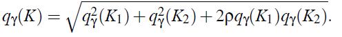
Consider two assets with returns 1+ξi, i = 1, 2, where ξ’s have a joint normal distribution, E{ξi} = 0, Corr{ξ1, ξ2} = ρ. Let Ki be the profit of an investment in the ith asset, and K be the total profit. Prove that
Take real data on the daily stock prices for the stocks of two companies for one year from, say, http://finance.yahoo.com or another similar site. Using the VaR criterion, for different values of γ, compare the performance of the companies. (The analysis should be based on returns, that is, on the
Let X1 and X2 be the returns of two securities with respective means m1 and m2, and variances σ21 and σ22 . We invest one unit of money: α in the first security and 1−α in the second. So, the investment return is the r.v. X = αX1 +(1−α)X2. Assume X1 and X2 to be independent.(a) Find an
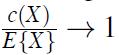
Let X be uniformly distributed on [0,1], and let Y take on values from [1, ∞), and P(Y > x) = 1/xα for all x ≥ 1 and some α > 2. This is a version of the Pareto distribution we discussed in Example 6.1.3-3 and Exercise 6.9. Verify that
Regarding the phenomenon we watched in Section 1.2.4, discuss to what extent the situation changes if we replace in (1.2.2) the standard deviation by the variance. In particular, consider the situation of Exercise 7.Exercise 7Let X be uniformly distributed on [0,1], and let Y take on values from
Let u1(x) and u2(x) be John’s and Mary’s utility functions, respectively. How do John’s and Mary’s preferences differ if(i) u1(x) = 2u2(x)+3; (ii) u1(x) = −2u2(x)+3?
Consider an EU maximizer with utility function u(x) = xα; 0 ≤ α < 1. (a) Find a certainty equivalent of a r.v. X1 =b>0 or 0 with respective probabilities p and q=1−p. (b) Compare it with the certainty equivalent of a r.v. X2 uniform on [0,b].Which certainty equivalent is larger for p = 1/2?
Consider a r.v. X such that P(X > x) = x−1 for x ≥ 1. (This is a particular case of the Pareto distribution.) Does X have a finite expected value? Does X have a finite certainty equivalent for u(x) = √x? If so, find it.
Consider the EUM criterion with the exponential utility function u(x) = −e−βx.(a) Show that if for some X and Y, we have X ≳ Y, then w+X ≳ w+Y for any number w. (The number w may be interpreted as the initial wealth, and X and Y as random incomes corresponding to two investment strategies.
Let X be exponential, and u(x) = −e−βx. Show that for the certainty equivalent c(X), we haveas E{X}→0, that is, c(X)≈ E{X} if E{X} is small. Interpret it considering u(x) for small x’s.
Provide calculations similar to those in Example 2.1-5 for w = 1 and ξ uniform on [0,1].
Compare the expected values and certainty equivalents for different values of α including the case α→0 and α→∞ . Interpret results.
A customer of an insurance company is an EU maximizer with a total wealth of 100. She/he is facing a random loss ξ for which P(ξ = 0) = 0.9, P(ξ = 50) = 0.05, P(ξ = 100) = 0.05.(a) Let the utility function of the customer be u(x) = x−0.005x2 for 0 ≤ x ≤ 100. Graph it. Why do we consider
Take real data on the daily stock prices for the stocks of two companies for one year from, say, http://finance.yahoo.com or another similar site. Considering a particular utility function, for instance, u(x) = −e−0.001·x, determine which company is better for an EU maximizer with this utility
Take real data on the daily stock prices for the stocks of two companies for one year from, say, http://finance.yahoo.com or another similar site. Considering a particular utility function, for instance, u(x) = −e−0.001·x, determine which company is better for an EU maximizer with this utility
(a) Is Condition Z from Section 2.3 a requirement on (i) distribution functions, or (ii) random variables, or (iii) the preference order under consideration?(b) Is Condition Z based on the concept of expected utility?
Is it true that for an expected utility maximizer to be a risk averter, his/her utility function should have a negative second derivative? Let u(x) = x for x ∈ [0,1], and u(x) = 1/2 + 1/2x for x ≥ 1. Graph this function. Is an EU maximizer with this utility function a risk averter? (Advice:
Check for risk aversion the criteria with utility functions from Section 2.2
Suppose that in the situation of Example 1.1-1, a person has preferred Y. Would you expect the same answer if we change units of money and compare, say, $50,000 and Y = $100,000 with probability 1/2? How may the utility function look in this case?
Let the utility function of a person be u(x) = eax, a > 0. Graph it. Is the person a risk averter or a risk lover? Show that in this case, the results of the comparison of risky alternatives does not depend on the initial wealth and has the additivity property for certain equivalents.
Let X be exponential, and u(x) = −e−βx. Show that the certainty equivalent c(X) → 0 as β→∞. Interpret it in terms of risk aversion.
Let Michael be an EU maximizer with utility function u(x) = −exp{−βx} and β = 0.001. (For this value of β, the values of expected utility in this problem will be in a natural scale.) Michael compares stocks of two mutual funds. The current price for each is $100 per share. Michael believes
Consider two r.v.’s both taking on values 1,2,3,4. For the first r.v., the respective probabilities are 0.1, 0.2, 0.5, 0.2, for the second, 0.1, 0.3, 0.3, 0.3. Which r.v. is better in the EUM-riskaversion case? Justify the answer.
Consider a r.v. taking values x1,x2, ...with probabilities p1, p2, ... , respectively. Let the xi’s be equally spaced, that is, xi+1 −xi equals the same number for all i. Assume that for a particular i, we replaced probabilities pi−1, pi, pi+1 by probabilities pi−1+Δ, pi−2Δ, pi+1+Δ
Find the certainty equivalent of a r.v. X = d > 0 or 0 with probabilities p and q, respectively. Analyze and interpret the case of p close to one.
Let g(s)defined in Section 3.2 equal 1−e−s for s > 0, and s for s ≤ 0. Graph g(s). Let c be the certainty equivalent of a r.v. X. Is it true that c≤E{X} ? Estimate the certainty equivalent for X equal to 1 or 0 with equal probabilities.
Let an individual’s preferences be described by the RDEU criterion with Ψ(p) = 1−(1− p)β. In other words, Ψ(p) is close to a power function for p close to one, that is, for p’s corresponding to large values of r.v.’s. Let X be an exponential r.v. with a distribution F. Show that in
Consider the RDEU scheme. Let F be the uniform distribution on [0,b], u(x) = xα, and Ψ(p) = pβ. Find a certainty equivalent and show that for β > 1 it is larger than for β = 1 (the expected utility case). Interpret this. Consider the case β < 1.
Jane is hiking in one of two areas; in both she may come across a rattlesnake. For the first area, the probability of seeing a rattle snake is 0.1, and for the second, it is 0.07. If Jane saw a rattle snake last time, she switches the areas; and if she did not see a snake, she keeps hiking in the
The Ehrenfest ball-box model. Consider a fixed number n of balls distributed somehow in two boxes. One at a time, a ball is selected at random from the total of n balls and moved from its box to the other. Let Xt be the number of balls in, say, the first box at step t.Originally, this model was
In a physical space, there is a site and particles are arriving at the site. At time moment t = 0, the site is vacant. At moments t = 1,2, ..., exactly one particle arrives with a probability of p1. If the site is vacant, the particle occupies the site. If the site is occupied, arriving particles
In the situation of Exercise 3, suppose that there are two sites, and the particles sitting in these sites exhibit independent behavior. Let Xt be the total number of particles in both sites.Show that Xt is a Markov chain and write its transition matrix.Exercise 3In a physical space, there is a
Consider the chain in Example 1.2-5 and set fk = P(ξi = k), k = 0,1, ... . (This probability is the same for all i). Find the transition matrix.Example 1.2-5Let Xt = max{ξ0, ξ1, ..., ξt}. Clearly,and (1.2.5) holds for g(m,n) = max{m,n}. In Exercise 5, it is suggested to the reader to find the
Show that the random walk process in Section 2.2.4 is a Markov chain. Find the transition matrices for the following two cases.(a) The process does not stop upon reaching any level. In this case, Xt may assume all values 0,±1,±2, ... .(b) The process comes to a stop when Xt = 0 or a, as it was
Show that the branching process from Section 4.1 is a Markov chain. Describe how the transition matrix may look.
For Example 1.2-1, compute the probability of the path 0→0→1, and the probability of the transition from state 0 to state 1 in two steps. Which probability is larger? Could we expect it without calculations?
We have mentioned that the Markov model in Example 1.2-1 may be too simple for describing the evolution of the weather conditions: in general, it is certainly useful to know the tendency of weather conditions in the past.However, we can keep using the Markov setup if we extend the set of possible
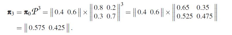
For the figure 57.5% at the end of Example 1.3-3 to be true, should we assume that the citizens are migrating independently?Example 1.3-3 We revisit Example in Section 1.1. Doing simple calculations or using software, we getThus, the probability that a randomly chosen citizen will live in area 0 at
It concerns the transition of individuals between social classes defined on the basis of income or occupation. Sociologists distinguish inter-generational mobility from parents’ class to child’s class and intra-generational mobility over an individuals life course. The particular model below
Provide an Excel worksheet for Example 1.2-4 and play a bit, changing the transition matrix and watching what happens. Consider several realizations, generating different random numbers.Example 1.2-4Concerns the simulation of Markov chains. A general simulation theory is presented in Section 7.4,
For the situation of Exercise 6b, in the case of the symmetric walk, let Tu be the random time it takes for the process to reach either level 0 or a. Find E{Tu} for a = 4 and u = 0,1,2,3, 4.Exercise 6bShow that the random walk process in Section 2.2.4 is a Markov chain. Find the transition
Let us revisit Exercise 11 and consider a family from the middle class. In which generation on the average will the descendants of this family at the first time belong to the upper class?Exercise 11It concerns the transition of individuals between social classes defined on the basis of income or
Let us come back to the weather-condition example in Section 2.3. Suppose that either the today weather conditions are normal, or it is rainy. Without any calculations, show that the icy-road conditions will appear on the tenth day on the average.
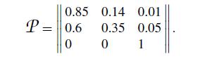
For a health insurance plan, for every client, the company distinguishes three conditions at the beginning of each year: “healthy”, “sick”, and “deceased”. The transition matrix isAssume that at the initial moment, 90% of the clients of the company are healthy.(a) Find the expected
Let us come back to Section 1.1. Suppose that in area 0, the living expenses of a citizen chosen at random is a r.v. with a mean of 10 (units of money) and a standard deviation of 1. For area 1, the corresponding characteristics are 9 and 2, respectively. Find the mean and standard deviation of the
Mr.M. runs a business. Each year, with a probability of 0.1, Mr.M. quits this business. Given that this does not happen, Mr. M. faces either “bad” or “good” year with respective average incomes 1 or 2. The transition probabilities for these two states are specified by the matrixwhere zero
In Exercise 1, using software or even a calculator, for a long period of time, estimate the proportion of the time when Jane hikes in the first area. Find the precise value.Exercise 1Jane is hiking in one of two areas; in both she may come across a rattlesnake. For the first area, the probability
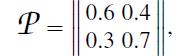
Each weekend Joan is either jogging or swimming. If Joan swam last weekend, she switches to jogging with probability 2/3. If she jogged, she jogs again with probability 1/2.(a) Find the proportions of the time Joan swims and jogs in the long run.(b) For the stationary regime, find the probability
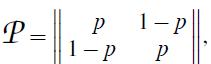
Let the transition matrix of a chain iswhere 0
Assuming that in Exercise 3, 0 < p1 < 1, 0 < p2 < 1, can we say without calculations whether the ergodicity property holds? Find the limiting distribution. What is happening when p1 gets smaller, very small? Explain the answer from a common-sense point of view.Exercise 3In a physical space, there
Setting in Exercise 4 p1 = p2 = 0.5, guess which the stationary probability, π0, π1, or π2, is the largest. Find these probabilities.Exercise 4In the situation of Exercise 3, suppose that there are two sites, and the particles sitting in these sites exhibit independent behavior. Let Xt be the
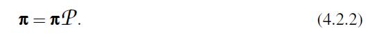
Consider Example 4.2-1 for k books. Show that in the long run, all k! permutations are asymptotically equally likely.Example 4.2-1Consider the process of random rearrangements with P given in (1.2.3). It is straightforward to verify that for such a matrix, equation (4.2.2) is true for π=(1/6, ...,
Let us revisit Exercise 2.(a) Explain why the limiting distribution does not exist.(b) Nevertheless, we can figure out the explicit pattern of the behavior of Xt. Using Excel or another software, for n = 4, compute Pt for, say, t = 2, ..., 8, and comment on the results. (P is a 5 × 5-matrix.)
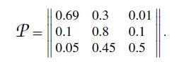
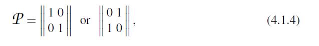
Show that the transition matrices in (4.1.4) do not satisfy Doeblin’s condition, while the matrix in Example 4.2-4 does.Example 4.2-4In a country, at the end of each year, the government arranges a poll where each interviewee evaluates her/his financial status as either “good,” or “fair,”
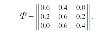
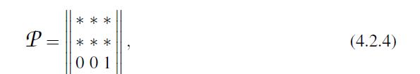
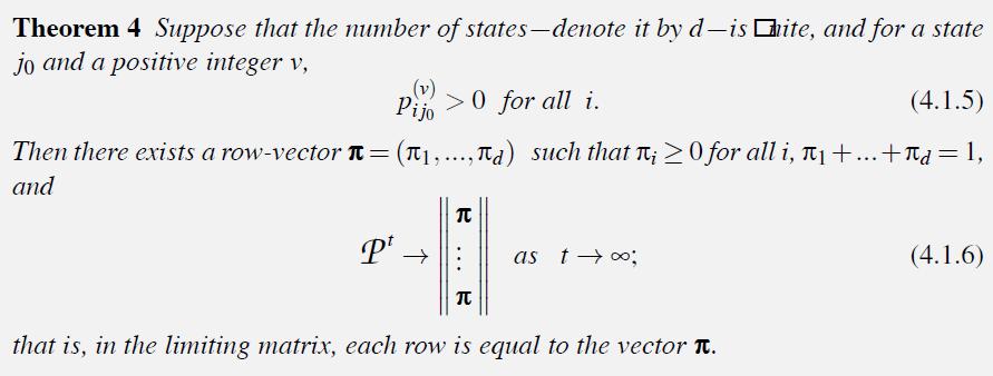
Does Doeblin’s condition of Theorem 4 hold for the transition matrix (4.2.4)? Connect it with what was said in Example 4.2-3.Example 4.2-3Let a chain have one absorbing state, say,where the stars ∗ represent positive numbers. The reader is invited to verify that in this case the solution to

Showing 6600 - 6700 of 6914

First
56
57
58
59
60
61
62
63
64
65
66
67
68
69
70

Step by Step Answers

Services

Sitemap
Fun
Definitions
Become Tutor
Used Textbooks
Study Help Categories
Recent Questions
Expert Questions
Campus Wear
Sell Your Books

Company Info

Security
Copyrights
Privacy Policy
Terms & Conditions
SolutionInn Fee
Scholarship
Online Quiz
Give Feedback, Get Rewards

Get In Touch

About Us
Contact Us
Career
Jobs
FAQ
Student Discount
Campus Ambassador

Secure Payment

Download Our App

© 2026 SolutionInn. All Rights Reserved