New Semester Started Get 50% OFF Study Help! --h --m --s Claim Now

Question Answers

Textbooks

Find textbooks, questions and answers

Oops, something went wrong!

Change your search query and then try again

Result Not Found

Books FREE
Study Help
Tutors
AI Study Planner NEW
Sell Books

Search
Sign In
Register

study help
business
probability and stochastic modeling

Applied Probability And Stochastic Processes 2nd Edition Frank Beichelt - Solutions

Let \(Y_{0}, Y_{1}, \ldots\) be a sequence of independent random variables with finite mean values. Show that the discrete-time stochastic process \(\left\{X_{0}, X_{1}, \ldots\right\}\) generated by\[X_{n}=\sum_{i=0}^{n}\left(Y_{i}-E\left(Y_{i}\right)\right)\]is a martingale.
Let a discrete-time stochastic process \(\left\{X_{0}, X_{1}, \ldots\right\}\) be defined by\[X_{n}=Y_{0} \cdot Y_{1} \cdots Y_{n}\]where the random variables \(Y_{i}\) are independent and have a uniform distribution over the interval \([0, T]\). Under which conditions is \(\left\{X_{0}, X_{1},
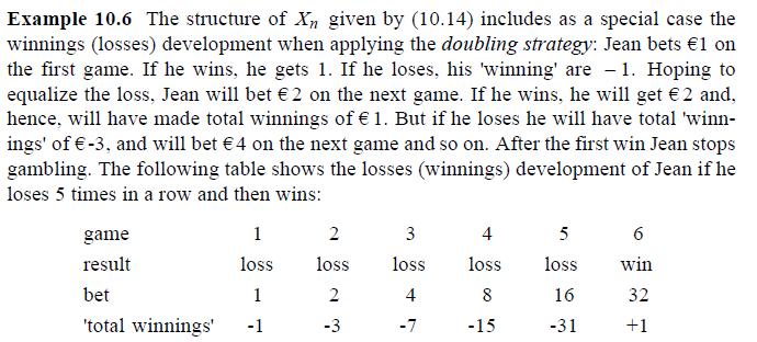
Determine the mean value of the loss immediately before the win when applying the doubling strategy, i.e., determine \(E\left(X_{N-1}\right)\) (example 10.6).Data from Example 10.6 Example 10.6 The structure of X given by (10.14) includes as a special case the winnings (losses) development when
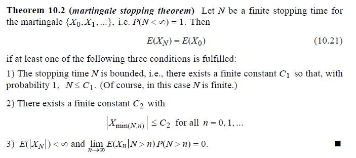
Why is theorem 10.2 not applicable to the sequence of 'winnings' \(\left\{X_{1}, X_{2}, \ldots\right\}\), which arises by applying the doubling strategy (example 10.6)?Data from Example 10.6Data from Theorem 10.2 Example 10.6 The structure of X given by (10.14) includes as a special case the
Jean is not happy with the winnings he can make when applying the 'doubling strategy'. Hence, under otherwise the same assumptions and notations as in example 10.6, he triples his bet size after every lost game, starting again with \(€ 1\).(1) What is his winnings when he loses 5 games in a row
Starting at value 0 , the profit of an investor increases per week by \(\$ 1\) with probbability \(p, p>1 / 2\), or decreases per week by one unit with probability \(1-p\). The weekly increments of the investor's profit are assumed to be independent. Let \(N\) be the random number of weeks until
Starting at value 0 , the fortune of an investor increases per week by \(\$ 200\) with probability \(3 / 8\), remains constant with probability \(3 / 8\), and decreases by \(\$ 200\) with probability \(2 / 8\). The weekly increments of the investor's fortune are assumed to be independent. The
Let \(X_{0}\) be uniformly distributed over \([0, T], X_{1}\) be uniformly distributed over \(\left[0, X_{0}\right]\), and, generally, \(X_{i+1}\) be uniformly distributed over \(\left[0, X_{i}\right], i=0,1, \ldots\).Verify: The sequence \(\left\{X_{0}, X_{1}, \ldots\right\}\) is a supermartingale
Let \(\left\{X_{1}, X_{2}, \ldots\right\}\) be a homogeneous discrete-time Markov chain with state space \(\mathbf{Z}=\{0,1, \ldots, n\}\) and transition probabilities\[p_{i j}=P\left(X_{k+1}=j \mid X_{k}=i\right)=\left(\begin{array}{c} n \\ j
Show that if \(L\) is a stopping time for a stochastic process with discrete or continuous time and \(0
Let \(\{N(t), t \geq 0\}\) be a nonhomogeneous Poisson process with intensity function \(\lambda(t)\) and trend function\[\Lambda(t)=\int_{0}^{t} \lambda(x) d x\]Check whether the stochastic process \(\{X(t), t \geq 0\}\) with \(X(t)=N(t)-\Lambda(t)\) is a martingale.
Show that every stochastic process \(\{X(t), t \in \mathbf{T}\}\) satisfying\[E(|X(t)|)
Verify that the probability density \(f_{t}(x)\) of \(B(t)\),\[f_{t}(x)=\frac{1}{\sqrt{2 \pi t} \sigma} e^{-x^{2} /\left(2 \sigma^{2} t\right)}, \quad t>0\]satisfies with a positive constant \(c\) the thermal conduction equation\[\frac{\partial f_{t}(x)}{\partial t}=c \frac{\partial^{2}
Determine the conditional probability density of \(B(t)\) given \(B(s)=y, 0 \leq s
Prove that the stochastic process \(\{\bar{B}(t), 0 \leq t \leq 1\}\) given by \(\bar{B}(t)=B(t)-t B(1)\) is the Brownian bridge.
Let \(\{\bar{B}(t), 0 \leq t \leq 1\}\) be the Brownian bridge. Prove that the stochastic process\[\{S(t), t \geq 0\} \text { defined by } S(t)=(t+1) \bar{B}\left(\frac{t}{t+1}\right)\]is the standard Brownian motion.
Determine the probability density of \(B(s)+B(t), 0 \leq s
Let \(n\) be any positive integer. Determine mean value and variance of\[X(n)=B(1)+B(2)+\cdots+B(n)\]
Check whether for any positve \(\tau\) the stochastic process \(\{V(t), t \geq 0\}\) defined by\[V(t)=B(t+\tau)-B(t)\]is weakly stationary.
Let \(X(t)=S^{3}(t)-3 t S(t)\). Prove that \(\{X(t), t \geq 0\}\) is a continuous-time martingale, i.e., show that\[E(X(t) \mid X(y), y \leq s)=X(s), \quad s
Show by a counterexample that the Ornstein-Uhlenbeck process does not have independent increments.
(1) What is the mean value of the first passage time of the reflected Brownian motion \(\{|B(t)|, t \geq 0\}\) with regard to a positive level \(x\) ?(2) Determine the distribution function of \(|B(t)|\).
Starting from \(x=0\), a particle makes independent jumps of length\[\Delta x=\sigma \sqrt{\Delta t}\]to the right or to the left every \(\Delta t\) time units. The respective probabilities of jumps to the right and to the left are\[p=\frac{1}{2}\left(1+\frac{\mu}{\sigma} \sqrt{\Delta t}\right)
Let \(\{D(t), t \geq 0\}\) be a Brownian motion with drift with paramters \(\mu\) and \(\sigma\). Determine \(E\left(\int_{0}^{t}(D(s))^{2} d s\right)\).
Show that for \(c>0\) and \(d>0\)\[P(B(t) \leq c t+d \text { for all } t \geq 0)=1-e^{-2 c d / \sigma^{2}}\]
At time \(t=0\) a speculator acquires an American call option with infinite expiration time and strike price \(x_{s}\). The price [in \$] of the underlying risky security at time \(t\) is given by \(X(t)=x_{0} e^{B(t)}\). The speculator makes up his mind to exercise this option at that time point,
The price of a unit of a share at time point \(t\) is \(X(t)=10 e^{D(t)}, t \geq 0\), where \(\{D(t), t \geq 0\}\) is a Brownian motion process with drift parameter \(\mu=-0.01\) and volatility \(\sigma=0.1\). At time \(t=0\) a speculator acquires an option, which gives him the right to buy a unit
The value (in \(\$\) ) of a share per unit develops, apart from the constant factor 10 , according to a geometric Brownian motion \(\{X(t), t \geq 0\}\) given by\[X(t)=10 e^{B(t)}, 0 \leq t \leq 120\]where \(\{B(t), t \geq 0\}\) is the Brownian motion process with volatility \(\sigma=0.1\).At time
The value of a share per unit develops according to a geometric Brownian motion with drift given by\[X(t)=10 e^{0.2 t+0.1 S(t)}, t \geq 0\]where \(\{S(t), t \geq 0\}\) is the standardized Brownian motion. An investor owns a European call option with running time \(\tau=1\) [year] and with strike
The random price \(X(t)\) of a risky security per unit at time \(t\) is\[X(t)=5 e^{-0.01 t+B(t)+0.2|B(t)|}\]where \(\{B(t), t \geq 0\}\) is the Brownian motion with volatility\[\sigma=0.04\]At time \(t=0\) a speculator acquires the right to buy the share at price \(\$ 5.1\) at any time point in the
At time \(t=0\) a speculator acquires a European call option with strike price \(x_{S}\) and finite expiration time \(\tau\). Thus, the option can only be exercised at time \(\tau\) at price \(x_{s}\) independently of its market value at time \(\tau\). The random price \(X(t)\) of the underlying
Show that\[E\left(e^{\alpha U(t)}\right)=e^{\alpha^{2} t^{3} / 6}\]for any constant \(\alpha\), where \(U(t)\) is the integrated standard Brownian motion:\[U(t)=\int_{0}^{t} S(x) d x, t \geq 0\]
For any fixed positive \(\tau\), let the stochastic process \(\{V(t), t \geq 0\}\) be given by\[V(t)=\int_{t}^{t+\tau} S(x) d x\]Is \(\{V(t), t \geq 0\}\) weakly stationary?
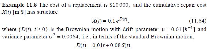
Let \(\{X(t), t \geq 0\}\) be the cumulative repair cost process of a system with\[X(t)=0.01 e^{D(t)}\]where \(\{D(t), t \geq 0\}\) is a Brownian motion with drift and parameters\[\mu=0.02 \text { and } \sigma^{2}=0.04\]The cost of a system replacement by an equivalent new one is \(c=4000\).(1) The
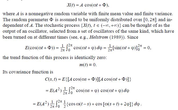
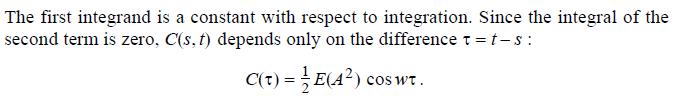
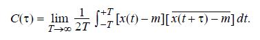
Define the stochastic process \(\{X(t), t \in \mathbf{R}\}\) by\[X(t)=A \cos (\omega t+\Phi)\]where \(A\) and \(\Phi\) are independent random variables with \(E(A)=0\) and \(\Phi\) is uniformly distributed over the interval \([0,2 \pi]\).Check whether the covariance function of the weakly
A weakly stationary, continuous-time process has covariance function\[C(\tau)=\sigma^{2} e^{-\alpha|\tau|}\left(\cos \beta \tau-\frac{\alpha}{\beta} \sin \beta|\tau|\right)\]Prove that its spectral density is given by\[s(\omega)=\frac{2 \sigma^{2} \alpha
A weakly stationary continuous-time process has covariance function\[C(\tau)=\sigma^{2} e^{-\alpha|\tau|}\left(\cos \beta \tau+\frac{\alpha}{\beta} \sin \beta|\tau|\right)\]Prove that its spectral density is given by\[s(\omega)=\frac{2 \sigma^{2}
A weakly stationary continuous-time process has covariance function\[C(\tau)=a^{-b \tau^{2}} \text { for } a>0, b>0\]Prove that its spectral density is given by\[s(\omega)=\frac{a}{2 \sqrt{\pi b}} e^{-\frac{\omega^{2}}{4 b}}\]
Define a weakly stationary stochastic process \(\{V(t), t \geq 0\}\) by\[V(t)=S(t+1)-S(t)\]where \(\{S(t), t \geq 0\}\) is the standard Brownian motion process.Prove that its spectral density is proportional to\[\frac{1-\cos \omega}{\omega^{2}}\]
A weakly stationary, continuous-time stochastic process has spectral density\[s(\omega)=\sum_{k=1}^{n} \frac{\alpha_{k}}{\omega^{2}+\beta_{k}^{2}}, \quad \alpha_{k}>0\]Prove that its covariance function is given by\[C(\tau)=\pi \sum_{k=1}^{n} \frac{\alpha_{k}}{\beta_{k}} e^{-\beta_{k}|\tau|}, \quad
A weakly stationary, continuous-time stochastic process has spectral density\[s(\omega)= \begin{cases}0 \text { for }|\omega|2 \omega_{0}, \\ a^{2} \text { for } & \omega_{0} \leq|\omega| \leq 2 \omega_{0},\end{cases}\]Prove that its covariance function is given by\[C(\tau)=2 a^{2} \sin
Let \(\mathbf{Z}=\{0,1\}\) be the state space and\[\mathbf{P}(t)=\left(\begin{array}{cc} e^{-t} & 1-e^{-t} \\ 1-e^{-t} & e^{-t} \end{array}\right)\]the transition matrix of a continuous-time stochastic process \(\{X(t), t \geq 0\}\). Check whether \(\{X(t), t \geq 0\}\) is a homogeneous Markov
A system fails after a random lifetime \(L\). Then it waits a random time \(W\) for renewal. A renewal takes another random time \(Z\). The random variables \(L, W\), and \(Z\) have exponential distributions with parameters \(\lambda, v\), and \(\mu\), respectively. On completion of a renewal, the
Consider a 1 -out-of- 2 system, i.e., the system is operating when at least one of its two subsystems is operating. When a subsystem fails, the other one continues to work. On its failure, the joint renewal of both subsystems begins. On its completion, both subsystems resume their work at the same
A copy center has 10 copy machines of the same type which are in constant use. The times between two successive failures of a machine have an exponential distribution with mean value 100 hours. There are two mechanics who repair failed machines. A defective machine is repaired by only one mechanic.
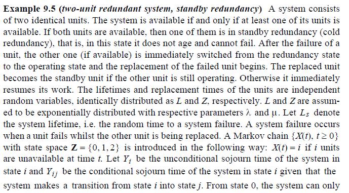
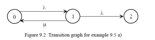
Consider the two-unit system with standby redundancy discussed in example 9.5 a) on condition that the lifetimes of the units are exponential with respective parameters \(\lambda_{1}\) and \(\lambda_{2}\). The other model assumptions listed in example 9.5 remain valid.Model the system by a Markov
Consider the two-unit system with parallel redundancy discussed in example 9.6 on condition that the lifetimes of the units are exponential with parameters \(\lambda_{1}\) and \(\lambda_{2}\), respectively. The other model assumptions listed in example 9.6 remain valid.Model the behavior of the
The system considered in example 9.7 is generalized as follows: If the system makes a direct transition from state 0 to the blocking state 2 , then the subsequent renewal time is exponential with parameter \(\mu_{0}\). If the system makes a transition from state 1 to state 2 , then the subsequent
Consider a two-unit system with standby redundancy and one mechanic. All repair times of failed units have an Erlang distribution with parameters \(n=2\) and \(\mu\). Apart from this, the other model assumptions listed in example 9.5 remain valid.(1) Model the system by a Markov chain and draw the
Consider a two-unit parallel system (i.e., the system operates if at least one unit is operating). The lifetimes of the units have an exponential distributions with parameter \(\lambda\). There is one repairman, who can only attend one failed unit at a time. Repairs times have an Erlang
When being in states 0,1 , and 2 , a (pure) birth process \(\{X(t), t \geq 0\}\) with state space \(\mathbf{Z}=\{0,1,2, \ldots\}\) has the respective birth rates\[\lambda_{0}=2, \lambda_{1}=3, \lambda_{2}=1\]Given \(X(0)=0\), determine the time-dependent state probabilities \(p_{i}(t)=P(X(t)=i)\)
Consider a linear birth process with state space \(\mathbf{Z}=\{0,1,2, \ldots\}\) and transition rates \(\lambda_{j}=j \lambda, j=0,1, \ldots\)(1) Given \(X(0)=1\), determine the distribution function of the random time point \(T_{3}\) at which the process enters state 3 .(2) Given \(X(0)=1\),
The number of physical particles of a particular type in a closed container evolves as follows: There is one particle at time \(t=0\). Its splits into two particles of the same type after an exponential random time \(Y\) with parameter \(\lambda\) (its lifetime). These two particles behave in the
A death process with state space \(\mathbf{Z}=\{0,1,2, \ldots\}\) has death rates\[\mu_{0}=0, \mu_{1}=2, \text { and } \mu_{2}=\mu_{3}=1\]Given \(X(0)=3\), determine \(p_{j}(t)=P(X(t)=j)\) for \(j=0,1,2,3\).
A linear death process \(\{X(t), t \geq 0\}\) has death rates \(\mu_{j}=j \mu ; j=0,1, \ldots\).(1) Given \(X(0)=2\), determine the distribution function of the time to entering state 0 ('lifetime' of the process).(2) Given \(X(0)=n, n>1\), determine the mean value of the time at which the process
At time \(t=0\) there are an infinite number of molecules of type \(a\) and \(2 n\) molecules of type \(b\) in a two-component gas mixture. After an exponential random time with parameter \(\mu\) any molecule of type \(b\) combines, independently of the others, with a molecule of type \(a\) to form
At time \(t=0\) a cable consists of 5 identical, intact wires. The cable is subject to a constant load of \(100 \mathrm{kp}\) such that in the beginning each wire bears a load of \(20 \mathrm{kp}\). Given a load of \(w k p\) per wire, the time to breakage of a wire (its lifetime) is exponential
Let \(\{X(t), t \geq 0\}\) be a death process with \(X(0)=n\) and positive death rates \(\mu_{1}, \mu_{2}, \ldots, \mu_{n}\).Prove: If \(Y\) is an exponential random variable with parameter \(\lambda\) and independent of the death process, then\[P(X(Y)=0)=\prod_{i=1}^{n}
A birth- and death process has state space \(\mathbf{Z}=\{0,1, \ldots, n\}\) and transition rates\[\lambda_{j}=(n-j) \lambda \text { and } \mu_{j}=j \mu ; j=0,1, \ldots, n\]Determine its stationary state probabilities.
Check whether or under what restrictions a birth- and death process with transition rates\[\lambda_{j}=\frac{j+1}{j+2} \lambda \text { and } \mu_{j}=\mu ; j=0,1, \ldots\]has a stationary state distribution.
A birth- and death process has transition rates\[\lambda_{j}=(j+1) \lambda \text { and } \mu_{j}=j^{2} \mu ; j=0,1, \ldots ; 0
Consider the following deterministic models for the mean (average) development of the size of populations:(1) Let \(m(t)\) be the mean number of individuals of a population at time \(t\). It is reasonable to assume that a change of the population size, namely \(d m(t) / d t\), is proportional to
A computer is connected to three terminals (for example, measuring devices). It can simultaneously evaluate data records from only two terminals. When the computer is processing two data records and in the meantime another data record has been produced, then this new data record has to wait in a
Under otherwise the same assumptions as in exercise 9.22, it is assumed that a data record, which has been waiting in the buffer a random patience time, will be deleted as being no longer up to date. The patience times of all data records are assumed to be independent, exponential random variables
Under otherwise the same assumptions as in exercise 9.22 , it is assumed that a data record will be deleted when its total sojourn time in the buffer and computer exceeds a random time \(Z\), where \(Z\) has an exponential distribution with parameter \(\alpha\). Thus, the interruption of the
A small filling station in a rural area provides diesel for agricultural machines. It has one diesel pump and waiting capacity for 5 machines. On average, 8 machines per hour arrive for diesel. An arriving machine immediately leaves the station without fuel if pump and all waiting places are
Consider a two-server loss system. Customers arrive according to a homogeneous Poisson process with intensity \(\lambda\). A customer is always served by server 1 when this server is idle, i.e., an arriving customer goes only then to server 2 , when server 1 is busy. The service times of both
A two-server loss system is subject to a homogeneous Poisson input with intensity \(\lambda\). The situation considered in exercise 9.26 is generalized as follows: If both servers are idle, a customer goes to server 1 with probability \(p\) and to server 2 with probability \(1-p\). Otherwise, a
A single-server waiting system is subject to a homogeneous Poisson input with intensity \(\lambda=30\left[h^{-1}\right]\). If there are not more than 3 customers in the system, the service times have an exponential distribution with mean \(1 / \mu=2[\mathrm{~min}]\). If there are more than 3
Taxis and customers arrive at a taxi rank in accordance with two independent homogeneous Poisson processes with intensities\[\lambda_{1}=4\left[h^{-1}\right] \text { and } \lambda_{2}=3\left[h^{-1}\right]\]respectively. Potential customers, who find 2 waiting customers, do not wait for service, but
A transport company has 4 trucks of the same type. There are 2 maintenance teams for repairing the trucks after a failure. Each team can repair only one truck at a time and each failed truck is handled by only one team. The times between failures of a truck (lifetime) is exponential with parameter
Ferry boats and customers arrive at a ferry station in accordance with two independent homogeneous Poisson processes with intensities \(\lambda\) and \(\mu\), respectively. If there are \(k\) customers at the ferry station, when a boat arrives, then it departs with \(\min (k, n)\) passengers (
The life cycle of an organism is controlled by shocks (e.g., accidents, virus attacks) in the following way: A healthy organism has an exponential lifetime \(L\) with parameter \(\lambda_{h}\). If a shock occurs, the organism falls sick and, when being in this state, its (residual) lifetime \(S\)
Customers arrive at a waiting system of type \(M / M / 1 / \infty\) with intensity \(\lambda\). As long as there are less than \(n\) customers in the system, the server remains idle. As soon as the \(n\)th customer arrives, the server resumes its work and stops working only then, when all customers
At time \(t=0\) a computer system consists of \(n\) operating computers. As soon as a computer fails, it is separated from the system by an automatic switching device with probability \(1-p\). If a failed computer is not separated from the system (this happens with probability \(p\) ), then the
A waiting-loss system of type \(M / M / 1 / 2\) is subject to two independent Poisson inputs 1 and 2 with respective intensities \(\lambda_{1}\) and \(\lambda_{2}\), which are referred to as type 1and type 2-customers. An arriving type 1-customer who finds the server busy and the waiting places
A queueing network consists of two servers 1 and 2 in series. Server 1 is subject to a homogeneous Poisson input with intensity \(\lambda=5\) an hour. A customer is lost if server 1 is busy. From server 1 a customer goes to server 2 for further service. If server 2 is busy, the customer is lost.
A queueing network consists of three nodes (queueing systems) 1,2 , and 3 , each of type \(M / M / 1 / \infty\). The external inputs into the nodes have respective intensities\[\lambda_{1}=4, \lambda_{2}=8, \text { and } \lambda_{3}=12 \text { [customers per hour]. }\]The respective mean service
A closed queueing network consists of 3 nodes. Each one has 2 servers. There are 2 customers in the network. After having been served at a node, a customer goes to one of the others with equal probability. All service times are independent random variables and have an exponential distribution with
Depending on demand, a conveyor belt operates at 3 different speed levels 1,2 , and 3. A transition from level \(i\) to level \(j\) is made with probability \(p_{i j}\) with\[p_{12}=0.8, p_{13}=0.2, p_{21}=p_{23}=0.5, p_{31}=0.4, p_{32}=0.6\]The respective mean times the conveyor belt operates at
The mean lifetime of a system is 620 hours. There are two failure types: Repairing the system after a type 1 -failure requires 20 hours on average and after a type 2 -failure 40 hours on average. \(20 \%\) of all failures are type 2 -failures. There is no dependence between the system lifetime and
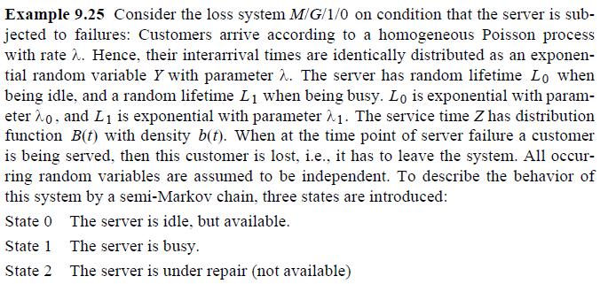
Under otherwise the same model assumptions as in example 9.25, determine the stationary probabilities of the states 0,1 , and 2 introduced there on condition that the service time \(B\) is a constant \(\mu\); i.e., determine the stationary state probabilities of the loss system \(M / D / 1 / 0\)
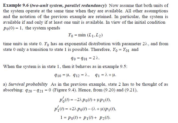
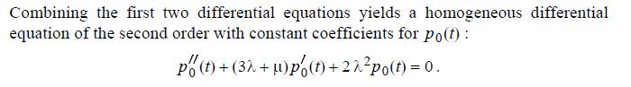
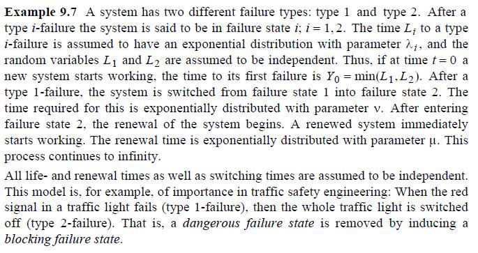
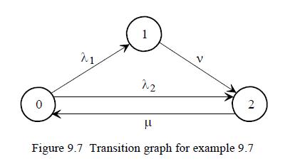
A system has two different failure types: type 1 and type 2 . After a type \(i\)-failure the system is said to be in failure state \(i ; i=1,2\). The time \(L_{i}\) to a type \(i\)-failure has an exponential distribution with parameter \(\lambda_{i} ; i=1,2\). Thus, if at time \(t=0 \mathrm{a}\)
The occurrence of catastrophic accidents at Sosal & Sons follows a homogeneous Poisson process with intensity \(\lambda=3\) a year.(1) What is the probability \(p_{\geq 2}\) that at least two catastrophic accidents will occur in the second half of the current year?(2) Determine the same probability
By making use of the independence and homogeneity of the increments of a homogeneous Poisson process with intensity \(\lambda\), show that its covariance function is given by\[C(s, t)=\lambda \min (s, t)\]
The number of cars which pass a certain intersection daily between \(12: 00\) and 14:00 follows a homogeneous Poisson process with intensity \(\lambda=40\) per hour. Among these there are \(2.2 \%\) which disregard the stop sign. The car drivers behave independently with regard to ignoring stop
A Geiger counter is struck by radioactive particles according to a homogeneous Poisson process with intensity \(\lambda=1\) per 12 seconds. On average, the Geiger counter only records 4 out of 5 particles.(1) What is the probability \(p_{\geq 2}\) that the Geiger counter records at least 2
The location of trees in an even, rectangular forest stand of size \(200 \mathrm{~m} \times 500 \mathrm{~m}\) follows a homogeneous Poisson distribution with intensity \(\lambda=1\) per \(25 \mathrm{~m}^{2}\). The diameters of the stems of all trees at a distance of \(130 \mathrm{~cm}\) to the
An electronic system is subject to two types of shocks, which occur independently of each other according to homogeneous Poisson processes with intensities\[\lambda_{1}=0.002 \text { and } \lambda_{2}=0.01 \text { per hour }\]respectively. A shock of type 1 always causes a system failure, whereas a
A system is subjected to shocks of types 1,2 , and 3 , which are generated by independent homogeneous Poisson processes with respective intensities per hour \(\lambda_{1}=0.2, \lambda_{2}=0.3\), and \(\lambda_{3}=0.4\). A type 1 -shock causes a system failure with probability 1 , a type 2 -shock
Claims arrive at a branch of an insurance company according a homogeneous Poisson process with an intensity of \(\lambda=0.4\) per working hour. The claim size \(Z\) has an exponential distribution so that \(80 \%\) of the claim sizes are below \(\$ 100000\), whereas \(20 \%\) are equal or larger
Consider two independent homogeneous Poisson processes 1 and 2 with respective intensities \(\lambda_{1}\) and \(\lambda_{2}\). Determine the mean value of the random number of events of process 2 , which occur between any two successive events of process 1 .
Let \(\{N(t), t \geq 0\}\) be a homogeneous Poisson process with intensity \(\lambda\).Prove that for an arbitrary, but fixed, positive \(h\) the stochastic process \((X(t), t \geq 0\}\) defined by \(X(t)=N(t+h)-N(t)\) is weakly stationary.
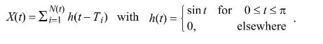
Let a homogeneous Poisson process have intensity \(\lambda\), and let \(T_{i}\) be the time point at which the \(i\) th Poisson event occurs. For \(t \rightarrow \infty\), determine and sketch the covariance function \(C(\tau)\) of the shot noise process \(\{X(t), t \geq 0\}\) given by N(t) X(t) =
Statistical evaluation of a large sample justifies to model the number of cars which arrive daily for petrol between 0:00 and 4:00 a.m. at a particular filling station by an inhomogeneous Poisson process \(\{N(t), t \geq 0\}\) with intensity function\[\lambda(t)=8-4 t+3 t^{2}\left[h^{-1}\right],
Let \(\{N(t), t \geq 0\}\) be an inhomogeneous Poisson process with intensity function\[\lambda(t)=0.8+2 t, \quad t \geq 0\]Determine the probability that at least 500 Poisson events occur in \([20,30]\).
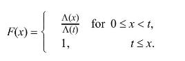
Let \(\{N(t), t \geq 0\}\) be a nonhomogeneous Poisson process with trend function \(\Lambda(t)\) and arrival time point \(T_{i}\) of the \(i\) th Poisson event.Given \(N(t)=n\), show that the random vector \(\left(T_{1}, T_{2}, \ldots, T_{n}\right)\) has the same probability distribution as \(n\)
Clients arrive at an insurance company according to a mixed Poisson process the structure parameter \(L\) of which has a uniform distribution over the interval \([0,1]\).(1) Determine the state probabilities of this process at time \(t\).(2) Determine trend and variance function of this process.(3)
A system is subjected to shocks of type 1 and type 2 , which are generated by independent Pólya processes \(\left\{N_{L_{1}}(t), t \geq 0\right\}\) and \(\left\{N_{L_{2}}(t), t \geq 0\right\}\) with respective trend and variance functions\[\begin{aligned} & E\left(N_{L_{1}}(t)\right)=t, \quad
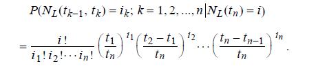
Prove the multinomial criterion (formula 7.55, page 280).Data from formula 7.55 P(NL(tk-1, tk)=ik; k = 1,2,...,n|N(tn) = 1) i! 11!12!in! ()" 71 12-11 12 tn in tn

Showing 5700 - 5800 of 6914

First
51
52
53
54
55
56
57
58
59
60
61
62
63
64
65
Last

Step by Step Answers

Services

Sitemap
Fun
Definitions
Become Tutor
Used Textbooks
Study Help Categories
Recent Questions
Expert Questions
Campus Wear
Sell Your Books

Company Info

Security
Copyrights
Privacy Policy
Terms & Conditions
SolutionInn Fee
Scholarship
Online Quiz
Give Feedback, Get Rewards

Get In Touch

About Us
Contact Us
Career
Jobs
FAQ
Student Discount
Campus Ambassador

Secure Payment

Download Our App

© 2026 SolutionInn. All Rights Reserved