New Semester Started Get 50% OFF Study Help! --h --m --s Claim Now

Question Answers

Textbooks

Find textbooks, questions and answers

Oops, something went wrong!

Change your search query and then try again

Result Not Found

Books FREE
Study Help
Tutors
AI Study Planner NEW
Sell Books

Search
Sign In
Register

study help
business
probability and stochastic modeling

Probability And Stochastic Modeling 1st Edition Vladimir I. Rotar - Solutions

Regarding Proposition 3, does the increase of the parameter α lead to the faster or slower rate of convergence to ±∞? Give a rigorous answer and a heuristic common-sense interpretation.
(a) Show that if in the normalization procedure (2.4.4), we divideby (cn)1/α, then the limiting distribution will be the distribution(b) Let X1, ...,Xn have the distributionsrespectively. Show that then max{X1, ...,Xn} has the distributionwith c = c1 +...+cn. One may say thatis stable with respect
Let X1, ...,Xn be independent standard exponential r.v.’s, andProve thatgrows as lnn; more precisely,where Vn is a r.v. whose d.f. P(Vn ≤ x) → G(x) = exp{−e−x}. This distribution is called the double exponential distribution. Graph the d.f. G(x). Is it the d.f. of a positive r.v.? Compare
Do Propositions 1 and 2 cover the situation of Exercise 10?Exercise 10Consider i.i.d. r.v.’s X1,X2, ... assuming a finite number of values x1 2 m. (a)Describe the behavior of the r.v.’sandheuristically.(b) Provide a rigorous explanation. How “fast” do the distributions of approach their
Suppose that in a country, for people who survived 30 years, the probability of dying before 40 years is negligible. How does the survival function look in this case?
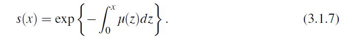
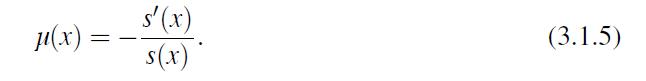
Show by differentiation that (3.1.7) is a solution to (3.1.5).
Is it true that a hazard rate function μ(x) is constant if and only if the distribution is exponential?
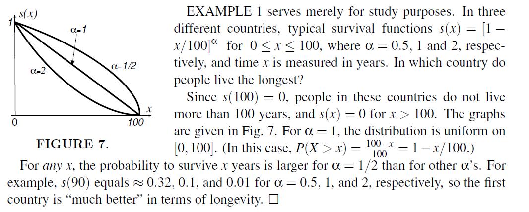
Find the force of mortality function for the cases of Example 3.1-1. Write s(120).
Find the hazard rate function μ(x) for the distribution uniform on [0,a]. What is limx→a μ(x)? Give a common-sense interpretation.
Find the survival functions for the Gompertz–Makeham andWeibull laws in Example 3.1-6.Example 3.1-6.Over the years, there has been a great deal of interest in finding analytical representations for survival functions of “real” people. Such attempts were based on the belief that the duration
Let μ(x) = (1+x)−1. Find the survival function. What is noteworthy?
(a) How should the mortality force change in order that the percent of newborns who will survive the first year will increase twice?(b) Do the same for the case of the first k years.
In a country, for a typical person of age 50, the probability to survive 80 years equals 0.5. Find the same probability for a country where(a) The force of mortality for people of age fifty and older is three times higher;(b) The force of mortality for people of age fifty and older is 0.01 less.
Consider the r.v. in Proposition 5. For P(W̴n ∞0 μi(x)dx = ∞ for all i = 1, ...,n? Give a rigorous proof and a common-sense explanation.
Prove that for X uniform on [0,a], the r.v. T(x) is uniformly distributed on [0,a−x]. Comment on this result.
Prove (3.2.3) rigorously. (Advice: You may start with t px =P(X >x+t |X >x)= P(X>x+t )/P(X>x) = P(X>x+1)/P(X>x) · P(X>x+t )/P(X>x+1) = P(X > x+1|X > x)P(X > x+t |X > x+1) = ....)
In a country, the survival function for women is closely approximated by sf(x) = (1 − x/100)1/2, while for men, it is sm(x) = (1−x/90)1/2. We assume that the probability of the birth of a boy is 1/2. Let Nm and Nf be the number of men and women of age x. Estimate E{Nf})E{Nm} for x = 0 and x =
(a) For young people, causes of death are related mostly to accidents. Proceeding from this, explain why the assumption of the approximate constancy of μ(x) may look reasonable for x’s between 30 and 40 years.(b) For what x’s do we need to know values of μ(x) to compute the probability that
Which is larger: the probability that a system will work 100 hours given that it has been working 50 hours or the same probability given that the system has been working 60 hours? State the question in general, using letters rather than numbers, and give a rigorous proof.(Advice: Show that t px =
In a city, homeowners use two types of heaters. The heaters of the first type constitute 30%, and their lifetimes are exponentially distributed with a mean of 10 years. The heaters of the second type are cheaper, and their lifetime is also exponential but the mean time is 8 years.Thus, the
For a r.v. |X| where X is standard normal, describe the behavior of the hazard rate μ(x) for large x’s.
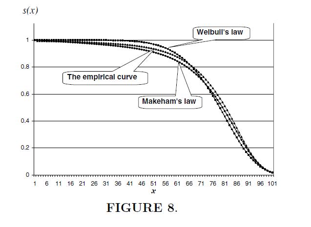
Proceeding from Fig. 8, argue that the phenomenon described, does not take place for a lower age; say, for x = 20, x = 50, or even for x = 60.
Consider a counting process Nt for which interarrival times are independent and uniform on [0,1]. Show that in this case(a) Increments of the process are dependent;(b) The process is not Markov. Does your answer to the second question answer the first? Give an answer to the first question
Let the independent exponential interarrival times in Example 2-1 be not identically distributed.Give an heuristic argument on whether the counting process Nt still have independent increments. Compare it with the case of identically distributed interarrival times. (Advice: Assume, for example,
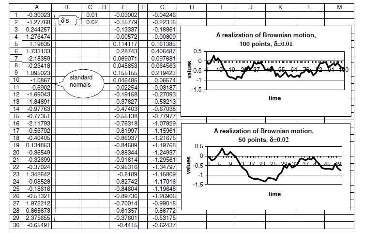
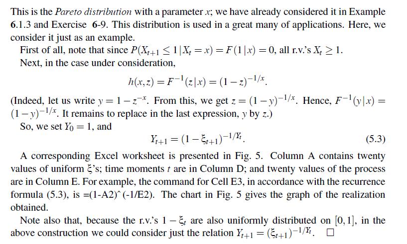
Provide an Excel worksheet with realizations of Brownian motion. Play a bit with it, considering—first of all—different normal values generated and different δ’s.
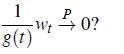
Show that 1/t wt P→ 0 as t → ∞. In other words, wt is growing slower than t. For which functions g(t) different from t it is also true; that is, when
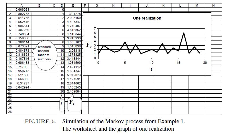
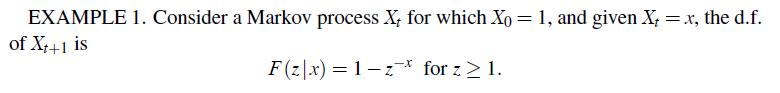
Using Excel, as we did in Example 5-1, or another software, simulate a realization of a Markov process Xt, t = 0,1, ..., such that X0 = 1, and given Xt = x, the r.v. Xt+1 is uniform on [ 1/1+x ,1].
Verify (1.1.3).
Customers arrive at a service facility according to a Poisson process with an average rate of 5 per hour. Find(a) The probabilities that (i) during 6 hours no customers will arrive, (ii) at most, twentyfive customers will arrive;(b) The probabilities that the waiting time between the third and the
How would you answer questions similar to those in Exercise 2 for the case where the mean interarrival time is 30 min.?Exercise 2Customers arrive at a service facility according to a Poisson process with an average rate of 5 per hour.
During an eight-hour work day, starting from 9am, customers of a company arrive at a Poisson rate of two per hour.(a) Assume that during the period from 10 am to 11 am, no customers arrived. Find the probability that during the next half an hour there will be no customers either.(b) Assume that
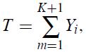
Let Nt be a Poisson process with a rate of λ, and let Ti be the time of the ith arrival. Write
Consider a homogeneous Poisson process Nt with a rate of λ. The time unit is an hour. Given that there were three arrivals during the first three hours, find the probability that(a) All three occurred during the first hour;(b) At least one arrival occurred during the first hour. Consider the
John is waiting for his date Mary at a street corner. People are passing by at a Poisson rate of λ per minute. Suppose that John’s waiting time is uniformly distributed on the interval from a to a+b minutes (say, from 5 to 35 minutes). Find the expected value and variance of the number of people
Ann is receiving telephone calls from customers of a company. Calls come at a Poisson rate of one each 15 min. Consider a time interval and the probability that there will be no more than one call during this interval. What length should the interval have for this probability to be greater than 0.8?
Suppose that the model of Section 1.2 is used for describing the flow of customers entering a store. We consider all t ∈ [0, ∞). Which function λ(t) should we choose if the store is open from 10am to 6pm, the intensity of arrivals equals c1 = 1 from 10 am to 2 pm, is linearly growing with a
For a non-homogeneous Poisson flow of customers, the intensity λ(t) during the first 8 hours is increasing as 10(t/8)2 [ending up with 10 customers/hour at the end of the period]. Find the expected value and the standard deviation of the number of customers during the whole period. Given that the
A flow of arrivals Nt is a non-homogeneous Poisson process with the periodical intensity λ(t) = | sin πt|. The unit of time is a day.(a) What is the intensity of arrivals at the end and at the beginning of each day? When is the intensity the largest?(b) What are the mean and variance of the
Give an example of an intensity λ(t) for which the probability that no arrival will ever occur is 1/e.
Let the intensity of a non-homogeneousPoisson process λ(t)=1 for t ∈ [0,1], and λ(t)=100 for t ∈ [1,2]. Explain heuristically and rigorously that the interarrival times τ1 and τ2 are dependent. (Advice: Consider the conditional distribution of τ2 given τ1 = a for, say, a= 1/2 and a = 1.)
In an area, the process of the occurrences of traffic accidents is a Poisson process with a rate of λ = 30 per day. The probability that a separate accident causes serious injuries is p = 0.1.The outcomes of different accidents are independent. Estimate the probability that during a month, the
Argue that the M/M/1 model is not appropriate for when the service times, though being random, are close to a positive and most probable number; say, as in a ticket booth.
Customers arrive at a service facility with one server according to a Poisson process with a rate of 5 per hour. The service times are i.i.d. exponential r.v.’s, and on the average, the server can serve 7 customers per hour. Suppose that the system is in the stationary regime.(a) What is the
In the long run, the mean proportion of time when the server in a M/M/1 system is idle, is 0.9. Find the arrival/service ratio. Find the same if 0.9 is the proportion of time when there is no queue.
For the M/M/1 scheme, find the variance of the number of particles in the system.
(a) For the scheme of Section 2.1, considering the stationary regime, graph the mean of Xt as a function of ρ.(b) Do the same for the standard deviation.
For the scheme M/M/1, show that the mean length of the queue, given that the server is busy, is equal to the mean number of particles in the system. Argue that the answer is not so surprising as it looks at first glance, showing that this is a special property of the process we consider. (Advice:
Consider the scheme M/M/1.(a) Does the mean number of customers in the queue increase or decrease when ρ is increasing?(b) Find P(Xt > k) in the stationary regime. Does this probability increase or decrease when ρ is increasing?(c) Argue that both your answers are consistent with the
Consider the M/M/1 model, and suppose that the server started to serve a new customer.(a) Find the probability that during the service time of a customer, no new customer will arrive. (Advice: Use conditioning.)(b) Do you expect the mean number of new customers who will arrive during the service
Consider theM/M/1 queueing model, and denote by T the amount of time a randomly chosen customer spends in the system. We consider the stationary regime and take for granted that the r.v. K, the number of customers that are ahead of a newly arriving customer, has the same distribution as Xt in the
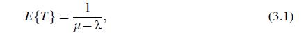
It may be proved that for μ>λ, the waiting time T defined in Exercise 23 has the exponential distribution with the parameter μ−λ. Argue that this is consistent with (3.1). For the situation of Exercise 16, compute the probability that the waiting time will exceed one hour. Suppose that in the
Consider the M/M/1 queueing model, and as in Exercise 23, take for granted that the r.v. K, the number of customers that are ahead of a newly arriving customer, has the same distribution as Xt in the stationary regime. Prove the fact that we use in Exercise 24. (Advice: Use the result of Example
Describe the behavior of the process Xt in Section 2.3 for (a) λ0 = λ1 = λ > 0, λk = 0 for all k ≥ 2, and μk = 0 for all k; (b) λ0 = λ1 = λ > 0, λk = 0 for all k ≥ 2, and μ0 = 0, μ1 = μ> 0, μ2 = 2μ.
Consider the M/M/1 scheme with a capacity of a.(a) Make sure that the limiting probabilities in (2.4.6) are positive for all ρ ≠ 1.(b) Figure out for which ρ the probability πk, as a function of k, is increasing (certainly, for k = 0, ...,a); for which ρ it is decreasing; and for which ρ
(a) For a M/M/1 service facility with a capacity of two, find π0, π1, π2 in two cases: (i) λ = 3, μ= 6 and (ii) λ = 6, μ= 3. Compare the results.(b) Establish a general pattern; namely, show that if π∗k is the limiting probability corresponding to the replacement of ρ with 1/ρ, then πk
Find the coefficient of variation for the number of particles in the system in the stationary regime for the M/M/∞ scheme with an arrival/service ratio of ρ.
In a large store, there are many cashier counters. Customers arrive at the checkout area at a Poisson rate of five per minute. The service times are independent and exponential with a mean of one minute. Let k be a number such that the probability that the number of busy counters exceeds k is not
Customers arrive at a single-server facility at a Poisson rate of λ; the service time is exponential with parameter μ. However, if a customer arrives when the server is busy and there are k people in line (k = 0,1, ... ), then the customer decides to wait with a probability of 1/(k+1). Find
Consider two queueing systems. The first has two servers; the service time for each is exponential with parameter μ. The second system has a single server whose service time is exponential with parameter 2μ; that is, the single server in the second system works twice as fast as each server in the
Make sure that the general formula for the steady-state distribution for the M/M/s system leads to the corresponding distributions for the particular cases s = 1 and s = ∞.
A receiver of “particles” has two cells each of which may contain only one particle. The cells are empty at the initial time. Particles arrive at a Poisson rate of λ. If one cell is occupied, no departures are possible. Once both cells are occupied, particles from outside do not enter the
Does Nt depend on τi’s? Give a particular example.
Which of the following is true? Compare with (1.1). Justify your answers.(a) Nt > n if and only if Tn < t;(b) Nt ≤ n if and only if Tn ≥ t;(c) Nt < n if and only if Tn > t.
Tourists arrive at a historic park (for simplicity, one at a time) according to a Poisson process at a rate of 40 per hour. Each five people take an excursion in a minivan. Let Nt be the number of excursions arranged by time t.(a) Show that Nt is a renewal process. What is the distribution of the
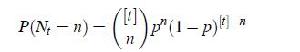
Let the interarrival times τi have a geometric distribution; namely, P(τi = m) = p(1− p)m−1 for m = 1,2, ... and a parameter p ∈ (0,1).(a) Show that Tn has a negative binomial distribution. With which parameters?(b) Show thatfor n ≤ [t], where [t] stands for the integer part of t.(c) Is
We have already considered the notion of the coefficient of variation σ/m of a r.v. X with a mean of m and a standard deviation of σ. Find the limit of the coefficient of variation for Nt as t →∞ and interpret your result.
Suppose that for a renewal process Nt, the interarrival times have the Poisson distribution with a mean of λ. Find the distribution of Tn and write a formula for P(N1 ≥ n). For which t an s is it true that P(Nt ≥ n) = P(Ns ≥ n)?
In a store, the inter-occurrence times of the replenishment of stock for a particular product are i.i.d. r.v.’s with a mean of five days and a standard deviation of one day. Each replenishment action costs $1500. Estimate the 0.95-quantile for the total replenishment expenses during a quarter;
Consider a renewal process Nt with i.i.d. interarrival times τi. Say, a piece of equipment serves until it breaks down; upon failure it is instantly replaced, and the renewal process continues.(a) Suppose we want to “inspect” the process, fixing a time t and observing the length of the
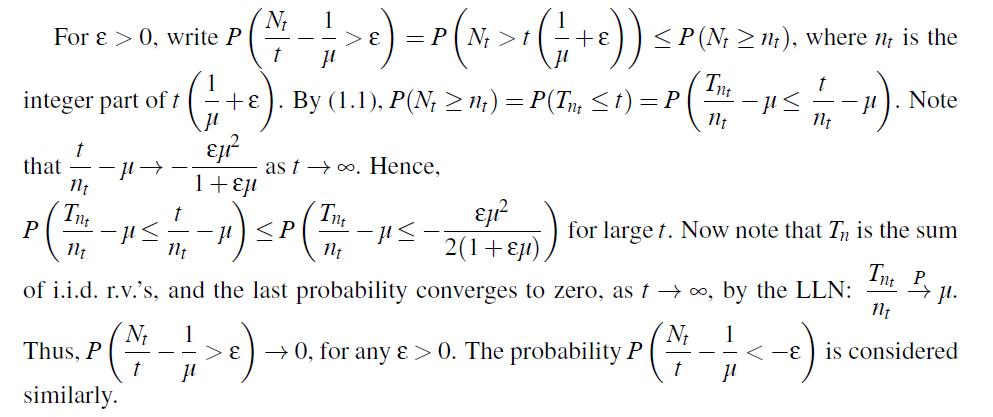
Prove thatproceeding from the following outline. For i.i.d. τ’s, set μ= E{τi} ≠ 0.
Estimate P(N60 = 25) in the situation. To what extent should we trust the estimate we obtained?
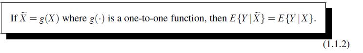
Prove (1.1.2) for the general mapping g(·).
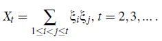
Let ξ1, ξ2, ... be i.i.d. r.v.’s with zero means. Set X0 = X1 = 0,Show that Xt is a martingale with respect to ξt.
Let ξ1, ξ2, ... be independent r.v.’s uniformly distributed on [0,a]. Let X0 = 1 and Xt =Ct ξ1 · ... · ξt. For which constant Ct is Xt a martingale?
Let ξ1, ξ2, ... be independent r.v.’s having an exponential distribution, and E{ξi} = 1. Let S0 = 0, St = ξ1 +...+ξt, and Xt = Ct exp{−St}, where Ct is a constant such that Xt is a martingale.(a) Find Ct.(b) Find limt→∞ Xt. How fast is such a convergence?
Show directly that in the urn model, the probability of selecting a red ball at the second drawing is the same as at the first.
Let ξ1, ξ2, ... be i.i.d. r.v.’s with zero mean and variance σ2 > 0, S0 = 0, St = ξ1+...+ξt for t = 0,1, .... Show that Xt = S2t −σ2t is a martingale with respect to ξt.
Let Xt = 2t ξ1 · ... · ξt, where ξ’s are independent and take on values 0 and 1 with equal probabilities. Show that Xt is a martingale. What is E{Xt}? What is limt→∞ Xt?
(a) Let ξ1, ξ2, ... be independent standard normal r.v.’s, S0 = 0, St = ξ1+...+ξt , X0 = 1, and Xt =Ct exp{St} for t = 1, ... . Find a constant Ct for which Xt is a martingale. Find limt→∞ Xt .How will the problem change if we consider Xt =Ct exp{−St}?(b) Do the same if ξ’s are
(a) Let ξ0, ξ1, ξ2, ... be independent r.v.’s and E{ξi} = 0 for all i. Let X0 = 0 and Xt = Z1+...+Zt for t ≥1 where Zk = ξk−1ξk. Are Z’s independent? Show that Xt is a martingale.(b)∗ Let E{ξi} = m = 0. Write Doob’s decomposition.
Let Xt be a branching process as it was defined in Sections 4.1, 3. Suppose that μ, the mean number of the off springs of a particular particle, is positive. (a) Show that the process Yt = 1/μt Xt is a martingale with respect to itself. (b) Show the same for the process Wt = uXt where u is the
Let ξ1, ξ2, ... be i.i.d. r.v.’s with a m.g.f. M(z), and St = ξ1 + ... + ξt. Show that Xt = M−t (z)exp{zSt} is a martingale with respect to ξt.
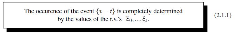
Let τ be an optional time as it was defined in (2.1.1).(a) Is the occurrence of event {τ > t} completely determined by the values of the r.v.’s ξ0, ..., ξt?(b) Explain why P(τ ∞t=0 P(τ = t).
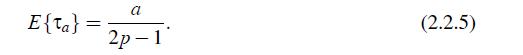
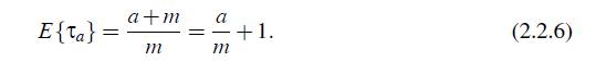
Explain why it takes considerably long to reach the level 1 starting from the neighbor level 0. Show that E{τa} > a if p < 1, not appealing to formula (2.2.5). What will happen if p is getting close to 1/2?
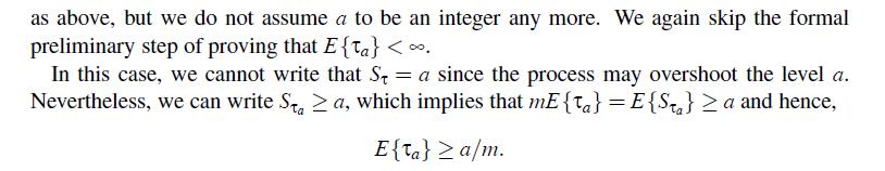
In the situation of Example 2.2-4, prove that E{τa} = ∞ if m = 0.
An alternative and direct proof of Wald’s identity (2.2.4) uses indicator r.v.’s It = 1 if τ ≥ k, and = 0 otherwise. Show that, in the notation of Proposition 5, Sτ = Σ∞k=1 ξkIk, and that the r.v.’s ξk and Ik are independent. Derive from this (2.2.4).
A gambler plays a game of chance favorable for him, winning in each play $5 with a probability of 0.55 and losing the same amount with probability 0.45. The gambler decides to play until the total gain will reach $100. Assuming that the gambler has sufficiently enough money at his disposal, find
Let S0 = 0, and a stopping time τ < c for a constant c with probability one. Using the optional stopping theorem, prove that E{S2τ} = σ2E{τ}. Compare it with the standard formula Var{St} = σ2t.
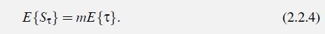
Consider a homogeneous Poisson process Nt with parameter λ. Show that the formula E{Nt} = λt is consistent with (2.2.6).
Consider the doubling strategy in the case of a game of roulette. Assume that a gambler always bets on red. Then at each play, the probability of success is p = 9/19 (there are 18 red, 18 black, and 2 green cells).(a) Is the profit Wt a martingale?(b) What will happen if after each failure, the
(a) Does the dimension of the price vector ψ equal the number of the assets in the market or the number of future states of nature?(b) Does the dimension of the trading strategy vector θ equal the number of assets in the market or the number of future states of nature?
Assume that in a country, there is a law which prohibits from selling short risky assets but allows one to borrow money with a fixed rate. When modeling such a market, what restrictions on the model of Section 3.2 should be imposed?
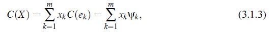
Assume that in a market, the pricing procedure (3.1.3) corresponds to the vector ψ = (0.2, 0.03, 0.07, 0.1, 0.2, 0.2).(a) How many states of nature can an investor face in this market?(b) Which states of nature do people consider in this case most likely, least likely?(c) If an investor borrows
The price of a stock is currently $50. It is expected that at the end of a time period, the price will be either $75 or $25. The risk-free interest over this period is zero.(a) Prove that there is no arbitrage opportunity. (b) Write the prices of call and put options with an exercise price of
Proceeding from a common-sense point of view, interpret the fact that the price of the European option is larger than the price of the American option.
Consider a stock whose initial price is $100, and each year the price either increases by 5% or drops by 6%. Let a risk-free interest be 4%.(a) Build a two-year tree for stock prices and determine a martingale measure. Is it unique? Find the probability corresponding to this measure (“the
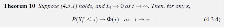
Show that Theorem 10 applies in the case of Example 4.3-2.
Let Xt , t = 0,1, ... , be a non-negative martingale, Mt = maxk≤t Xk. Show that for any t and x > 0,
Consider a symmetric random walk: X0 = u and Xt = u+ξ1+...+ξt, for t = 1,2, ..., where an integer u > 0 and ξ’s are independent and assume the values ±1 with equal probabilities. Let τ be the moment of ruin, that is, τ = min{t : Xt = 0}. Let Yt = Xt if t ≤ τ, and Yt = 0 if t ≥ τ. We
Provide an Excel worksheet illustrating the invariance principle of Section 1.1.2. To do this, simulate values of some independent r.v.’s, for example, exponential or uniform, construct sums Sk, and then the process Xt(n) (consider only points t = k/n). Provide charts with the graphs of

Showing 6500 - 6600 of 6914

First
56
57
58
59
60
61
62
63
64
65
66
67
68
69
70

Step by Step Answers

Services

Sitemap
Fun
Definitions
Become Tutor
Used Textbooks
Study Help Categories
Recent Questions
Expert Questions
Campus Wear
Sell Your Books

Company Info

Security
Copyrights
Privacy Policy
Terms & Conditions
SolutionInn Fee
Scholarship
Online Quiz
Give Feedback, Get Rewards

Get In Touch

About Us
Contact Us
Career
Jobs
FAQ
Student Discount
Campus Ambassador

Secure Payment

Download Our App

© 2026 SolutionInn. All Rights Reserved