New Semester Started Get 50% OFF Study Help! --h --m --s Claim Now

Question Answers

Textbooks

Find textbooks, questions and answers

Oops, something went wrong!

Change your search query and then try again

Result Not Found

Books FREE
Study Help
Tutors
AI Study Planner NEW
Sell Books

Search
Sign In
Register

study help
computer science
systems analysis and design 12th

Water Systems Analysis Design, And Planning Urban Infrastructure 1st Edition Mohammad Karamouz - Solutions

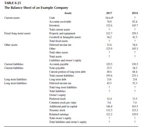
Derive cash flow statement from the given balance sheet (Table 8. 25) and income statement of a firm (Table 8. 26). Then, complete the balance sheet and check it. Analyze the financial position of the firm. Write your assumptions if there are any. Present the details of your computations. (Hint:
A water pump currently has a resale value of $25,000 and is estimated to have a resale value of $18,000 in 1 year’s time. The operating and maintenance cost of the pump for the coming year is $3,500, assumed to be incurred at the end of the year. The life cycle equivalent annual cost of a new
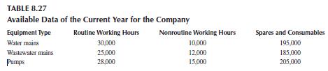
A company maintains a large network of water and wastewater equipment throughout a city. You are creating a maintenance budget for the coming year. Table 8. 27 shows the data available for the current year.The direct working cost rate is $30/hour with a multiplier for on-costs and overheads of 2.
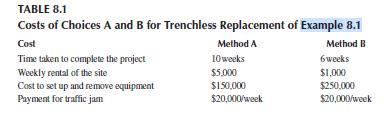
There are two choices, A and B, for the trenchless replacement of mains in an urban water distribution system (WDS). A $20,000 per week should be paid to the traffic control authorities for traffic jams during the project. The other costs of the two trenchless replacement methods are summarized in
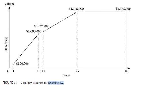
A wastewater collection network project in a city produces benefits, as expressed in Figure 8.1 :the $100,000 profit in year 1 is increased in 10 years on a uniform gradient to $1,000,000. Then it reaches $1,375,000 in year 25 with a uniform gradient of $25,000/year and it remains constant at
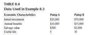
Two different types of pumps (A and B) can be used in a pumping station of an urban WDS. The costs and benefits of each of the pumps are displayed in Table 8.4 . Compare the two pumps economically using the MARR = 10% and considering that the time period of the study is equal to 12 years. TABLE 8.4
Assume that the annual costs of operation and maintenance of pumps A and B are equal to $4,000 and $6,000, respectively. Compare the two pumps from an economic aspect, using the benefit–cost ratio method.
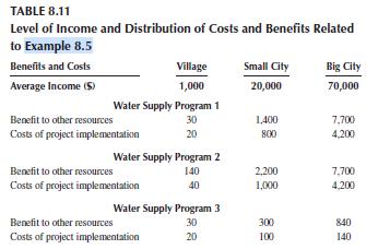
Three water supply projects are implemented in a region. Water demand of a big city, a small city, and a village will be supplied through these projects. Level of income and distribution of the costs and benefits for these projects are presented in Table 8.11 . Implementation of these projects
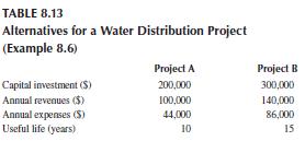
Consider two mutually exclusive alternatives for a water main distribution project, given in Table 8.13 . Assume that a study period of 15 years is applicable. Using the annual worth and PW methods, determine the preferred project. TABLE 8.13 Alternatives for a Water Distribution Project (Example
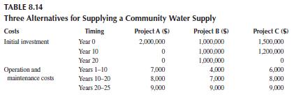
The three alternatives described in Table 8.14 are available for wastewater treatment of an urban area for the next 25 years of their life span. Using 5% discount rate, compare the three projects with the PW method. TABLE 8.14 Three Alternatives for Supplying a Community Water Supply Costs Timing
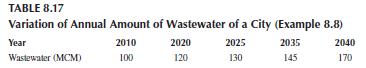
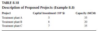
The variation of annual wastewater generation of a city over a 30-year planning time horizon is tabulated in Table 8.17 . Assume that the wastewater generation of this city in the year 2003 was about 90 MCM. Three projects have been proposed to treat wastewater projected generation until 2040. As
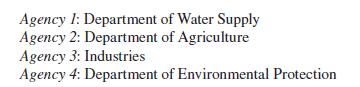
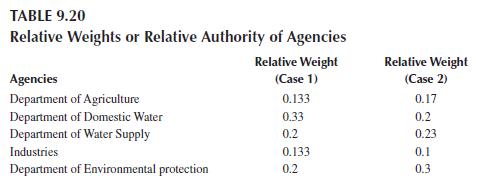
In an unconfined aquifer system, the following agencies are affected by the decisions made to discharge water from the aquifer to fulfill water demands:Department of Water Supply has a twofold role, namely, to allocate water to different purposes and to control the groundwater table variations. The
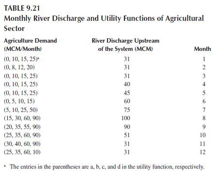
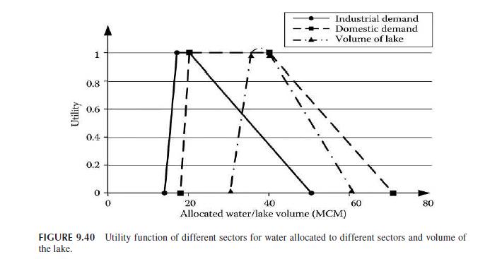
Determine the monthly water allocation to domestic, industrial, agricultural, and recreation demands in a river system shown in Figure 9. 39 The average monthly river discharges upstream of the system, in a 2-year time horizon, are presented in Table 9. 21.The return flow of domestic and industrial
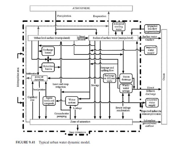
In Figure 9. 41, a typical dynamic model of urban water management has been shown.Using your own city data, create this model with system dynamic simulation software.Explain the relations you have considered between different parts of the urban water system. Discuss the future of water if water
Considering the urban water dynamic model in Figure 9. 41, what are the main parts of urban water system? How are different parts of the urban water supply affected by each other? Metropolitan area Precipitation ATMOSPHERE Evaporation Industrial cooling water Urban land surface (manipulated) Direct
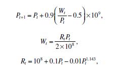
Formulate a population growth model in an urban area using an objective-oriented model/software based on the following data:• The initial value of “Population” is 50,000 people. “Population” increases at the rates of “Births” and “In Migration” and decreases at the rates of
Develop an urban growth model by considering the dynamics of population and business growth within a fixed area of a city based on the following assumptions. The model should contain two sectors: the “Business Structures” and the “Population” sectors.A city’s life cycle is characterized
Based on Problems 5 and 6, formulate a simple model to explain growth and stagnation in an urban area using an objective-oriented model/software based on the following data assumed for the urban area:In spite of dynamics considered in Problem 5, the rate of “In Migration” is also a product of
Using the data given in Problem 7, map the two interacting sectors of the “Business Structures” and the “Population” in an objective-oriented model/software.Data from problem 7 Based on Problems 5 and 6, formulate a simple model to explain growth and stagnation in an urban area using an
In Problem 7, what causes the growth of “Population” and “Business Structures” of an urban area during the early years of its development? Use the structure of model developed in the Problem 7 to answer this question. How does this answer compare to the answer in Problem 8?Data from problem
In Problem 7, what is the behavior of “Labor Availability” during the time horizon? What causes this behavior?Data from problem 7 Based on Problems 5 and 6, formulate a simple model to explain growth and stagnation in an urban area using an objective-oriented model/software based on the
In Problem 7, how does the finite “Land Area” limit the population growth? Will all the available “Land Area” be occupied in equilibrium condition (20 km2)? Use the model to show the effects of annexing surrounding land to increase the “Land Area” to 30 km2.Initialize the model in
In Problem 7, does the assumption of a fixed “Land Area” invalidate the model? Most cities can and have expanded from their original areas. How does such expansion influence the results given by the model? For example, what would be the likely consequences of expanding the “Land Area”
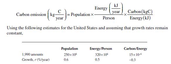
Consider the following disaggregation of carbon emissions:a. Find the carbon emission rate in 2030.b. Find the carbon emitted in those 40 years. kJ Energy year Carbon emission kg- = Population X- year Person Carbon (kgC) Energy (kJ) Using the following estimates for the United States and assuming
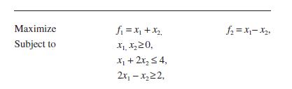
14- Consider the following problem with two objective functions:i. Represent graphically the decision space. ii. Display graphically the criteria space. Maximize Subject to f =x+x x0. x+2x4, 2x-x2,
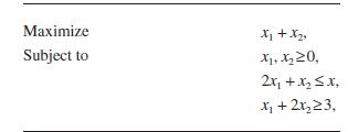
Consider the following linear programming problem:where ξ is randomly distributed with μ = 3 and σ2 = 1. Give the chance constraint formulation of the problem, and find the optimal solution.Consider a reservoir that supplies water to a city. The monthly water demand of this complex is 20
Find the minimum point of the function f (x) = 2x2 − 3x + 2 in the [−2, 2] interval using the GA.
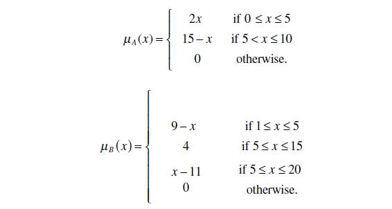
Fuzzy sets A and B are defined in X = [−∞, ∞], by the membership functions as follows:Determine the membership functions of A ∩ B, A ∩ B, AB, and A + B fuzzy sets. 2x if 0 x 5 H(x)= 15-x if 5 < x 10 0 otherwise. 9-x if 1x5 HB(x)=. 4 if 5 x 15 x-11 if 5 x 20 0 otherwise.
Solve Example 8. 2 with the changes assumed in Problem 8.Data from example 8. 2 A wastewater collection network project in a city produces benefits, as expressed in Figure 8. 1:the $100,000 profit in year 1 is increased in 10 years on a uniform gradient to $1,000,000. Then it reaches $1,375,000 in
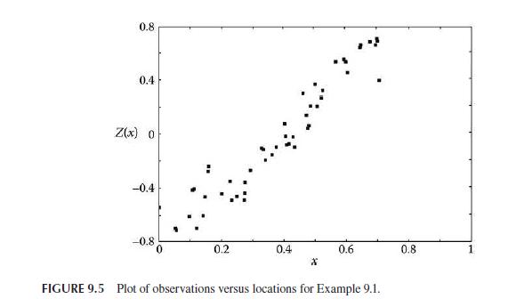
Consider 70 measurements that were synthetically generated from a one-dimensional random process (see Figure 9.5 ). Infer the variogram and test the intrinsic model. 0.8 0.4 Z(x) 0 -0.4 0.2 0.4 0.6 0.8 X FIGURE 9.5 Plot of observations versus locations for Example 9.1.
Consider a one-dimensional function with variogram γ(h) = 1 + h, for h > 0, and three measurements, at location x1 = 0, x2 = 1, and x3 = 3. Estimate the value of the function in the neighborhood of the measurement points, at location x0 = 2.
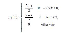
Consider fuzzy set A defined in X = [−2, 2] as follows:Determine the membership function of the fuzzy set induced by the function f (x) = x2. 2+x if -2x0, 2 2-x HA(x)= if 0
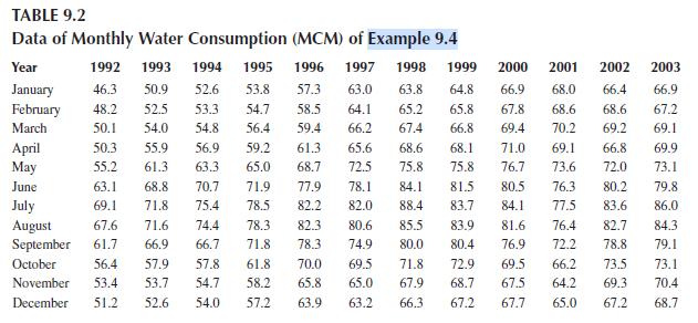
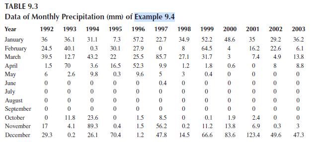
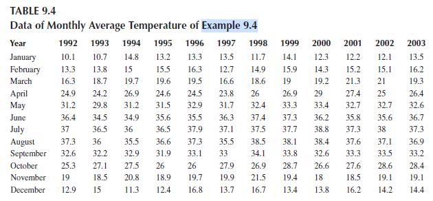
The studies in a city have shown that water consumption is a function of three climatic variables, including precipitation, weather humidity, and average temperature. The monthly data of water consumption, monthly rainfall, monthly average humidity, and temperature of this city are given in Tables
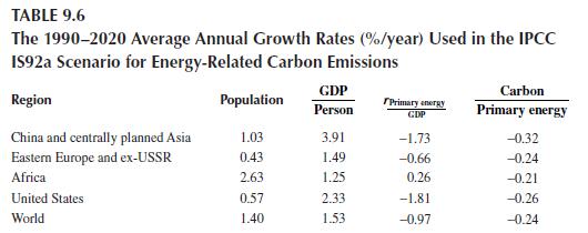
Emissions from fossil-fuel combustion in 2010 are estimated to be 7.6 GtC/year. In the same year, atmospheric CO2 concentration is estimated to be 390 ppm. Assume the atmospheric fraction remains constant at 0.38 .a. Assuming the energy growth rates shown in Table 9.6 , estimate the energy-related
Consider a city with limited resources and without any possibility for water transfer from adjacent basins. The quantity of surface and groundwater resources and their supply potential for domestic usage deteriorate because of the urban development and water quality problems caused by wastewater,
There are three methods for wastewater treatment in an urban area. The methods remove 1.2 , 2.5 , and 4 g/m3 amounts of the pollutants, respectively. The third technology is the best, but because of some limitations in allocating enough area, it cannot be applied to more than 40% of the wastewater
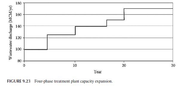
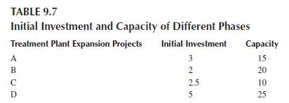
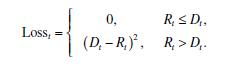
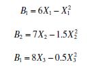
Based on the population growth analysis, a city’s wastewater is estimated to increase over time, as depicted in Figure 9.23 . Four phases for treatment plant expansion capacity are studied for the treatment of the future wastewater of this city in a 20-year planning time horizon. The capacity and
Assume a reservoir that supplies water for an urban area. The monthly water demand of this urban area (Dt) is about 10 million cubic meters. The total capacity of the reservoir is 30 million cubic meters. Let St (reservoir storage at the beginning of month t) take the discrete values 0, 10, 20, and
Find the maximum point of the function f(x) = 2x − x2 in the [0, 2] interval using the GA.
Find the best allocations of water to the three water-consuming firms using a genetic algorithm.The maximum allocation to any single user cannot exceed 5, and the sum of all allocations cannot exceed the value of Q, say 6. Only integer solutions are to be considered. The objective is to find each
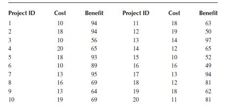
Consider the following water resource projects with the respective costs and benefits indicated.The total budget is 150 units. Determine the optimal portfolio of projects using the GA technique. Project ID Cost Benefit Project ID Cost Benefit 1 10 23456 18 94 11 18 63 94 12 19 50 10 56 13 14 97 20
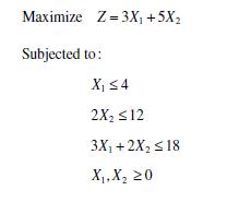
Calculate the following optimization answer using the Tabu method. Maximize Z=3X+5X2 Subjected to: X 4 2X2 12 3X+2X2 18 X,X 20
Assume that a combination of three alternative technologies removes two pollutants. They remove 3, 2, and 1 g/m3, respectively, of the first kind of pollutant and 2, 1, and 3 g/m3 of the second kind. If 1,000 m3 of each pollutant has to be treated in a day, determine the optimal combination of
Consider a multipurpose reservoir upstream of an urban area with conflicting objectives. Discuss the general considerations in resolving conflicts over a multipurpose reservoir operation.
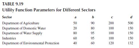
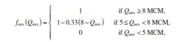
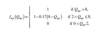
In Example 9.16 , consider the following data that show the demand and the utility function for different sectors that are obtained from compromising sessions. If the relative weights of agriculture, domestic water use, industrial water use, environmental protection, and power generation are
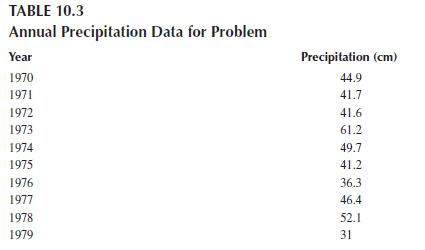
Calculate the sample mean, sample standard deviation, and sample coefficient of skewness of the annual precipitation data given in Table 10. 3. TABLE 10.3 Annual Precipitation Data for Problem Year 1970 Precipitation (cm) 44.9 1971 41.7 1972 1973 1974 1975 1976 1977 41.6 61.2 49.7 41.2 36.3 46.4
Consider the 100-year flood (P = 0. 01).a. What is the probability that at least one 100-year flood will occur during the 50-year lifetime of a flood control project?b. What is the probability that the 200-year flood will not occur in 50 years? In 100 years?c. In general, what is the probability of
A cofferdam has been built to protect homes in a floodplain until a major channel project can be completed. The cofferdam was built for the 40-year flood event. The channel project will require 5 years to complete. What are the probabilities thata. The cofferdam will not be overtopped during the 5
During a year, about 150 independent storm events occur in two cities, and their average duration is 6. 4 hours. Ignoring seasonal variations, in a year of 8,760 hours,a. Estimate the average time interval between two storms.b. What is the probability that at least 5 days will elapse between
Determine the hydrologic risk of a roadway culvert with 25 years of expected service life designed to carry a 50-year storm.
Construct the CDF of failure occurrences in two hazard rate situations: (a) ρ(t) = tα; and(b) ρ(t) = et − 1.
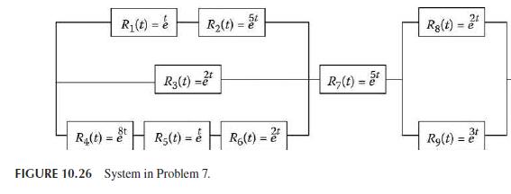
Calculate the system’s reliability shown in Figure 10. 26 at t = 0. 5 using reliability functions of system components. R(t) = R(t) R3(1)=2 t | R4(t) = || R(t) = || R(t) = ? | FIGURE 10.26 System in Problem 7. R(t)=5t R8(t) = 2 3r Rg(t) = e
Determine the hydrologic risk of a roadway culvert flooded with 50 years of expected service life designed to carry a 100-year storm.
Explain the stated case study in terms of probability distributions.
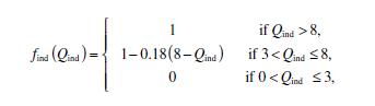
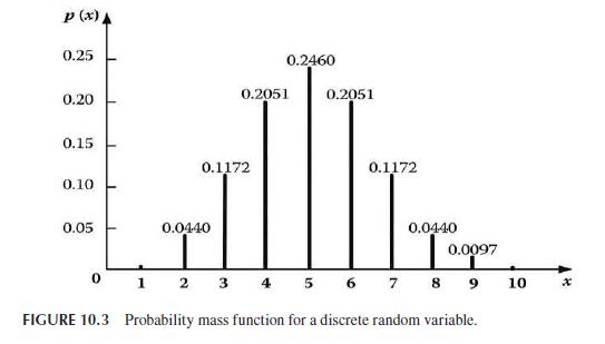
The probability mass function of floods is shown in Figure 10.3 . Estimate the mean number of floods in a 10-year period where f(x0) = f(x10) = 0.0010. P(x) 0.25 0.20 0.2051 0.2460 0.2051 0.15 0.1172 0.1172 0.10 0.05 0.0440 0.0440 0.0097 0 2 3 4 5 6 7 8 9 10 x FIGURE 10.3 Probability mass function
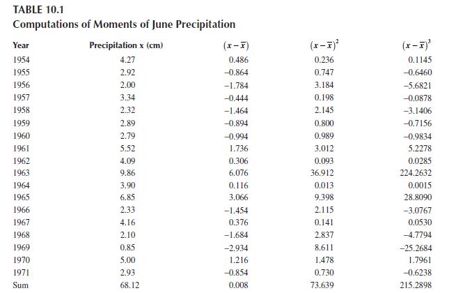
Estimate the mean, variance, standard deviation, and skew of 18-year precipitation data on a small basin given in Table 10.1 . TABLE 10.1 Computations of Moments of June Precipitation Year Precipitation x (cm) (x-x) (x-x) (x-x) 1954 4.27 0.486 0.236 0.1145 1955 2.92 -0.864 0.747 -0.6460 1956 2.00
What is the magnitude of the 100-year flood for a river 4.14 cubi(Q̅ = 4.14 cubic meter per second (cms), SQ = 3.31 cms and Cs 1.981 s cm using the gamma-3 and gamma-2 distribution?
Consider the 50-year flood (p = 0.02).a. What is the probability that at least one 50-year flood will occur during the 30-year lifetime of a flood control project?b. What is the probability that the 100-year flood will not occur in 10 years? In 100 years?c. In general, what is the probability of
A cofferdam has been built to protect homes in a floodplain until a major channel project can be completed. The cofferdam was built for a 20-year flood event. The channel project will require 3 years to complete. Hence, the process is B(3, 0.05). What are the probabilities thata. The cofferdam will
Determine the design return period, if the acceptable hydrologic risk is 0.15 (or 15%) during the 25-year lifetime of a culvert.
Assume the time between drought occurrences in a watershed follows the Weibull distribution.Formulate the reliability and hazard rate of this watershed in dealing with droughts.
10. 8 Construct the CDF of failure occurrences in two given situations: (a) The hazard rate is constant, ρ(ί) = α; and (b) ρ(t) = αβtβ − 1.
The system illustrated in Figure 10.9 includes five components, where components 2, 3, and 5 are parallel. Calculate the system reliability at t = 0.1 assuming that R1(t) = R4(t) = e−2t and R(t)= R(t)= R(t)=e(1i 2, 1 j 3).
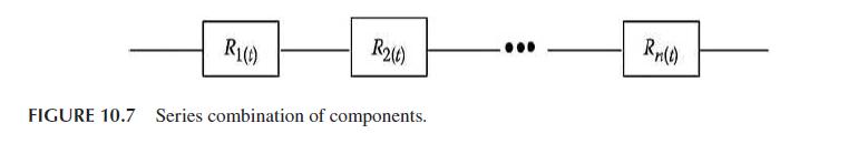
Evaluate the reliability of the water distribution network of Example 10.10 using the minimum cut-set method.Data from example 10.10 Calculate the system reliability of the water distribution network shown in Figure 10.7 considering that node 1 is the source node and nodes 3, 4, and 5 are demand
Calculate the reliability of the water distribution network of Example 10.10 using the tie-set method.Data from example 10.10 Calculate the system reliability of the water distribution network shown in Figure 10.7 considering that node 1 is the source node and nodes 3, 4, and 5 are demand nodes.
Develop a decision tree for evaluating the effect of a flood warning system development for$20,000 on the flooding mitigation. The probability of flooding is 0.1, and the damage associated with flooding in the absence of the warning system is $50,000. However, it is reduced to $5,000 with the flood
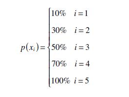
Let xi be the uncertain variable of rainfall depth of event i with the uncertain distribution of inundation probability as follows:Using the entropy definition for a discrete random variable, and assuming b = 10 as the logarithm base, calculate the entropy of x. [10% i=1 30% i=2 p(x)=50% i=3 70%
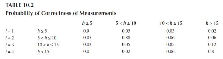
In order to drill a well, the water depth needs to be known. In preliminary designs, water depth is divided into four categories: less than 5 m, between 5 and 10 m, between 10 and 15 m, and more than 15 m. The following assumptions are known based on the experiences of the hydrology of the area:The
Construct the CDF of failure occurrences in two given situations. (1) ρ(t) = αt, and(2) ρ(t) = et.
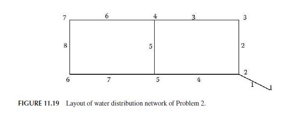
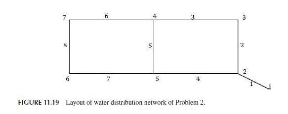
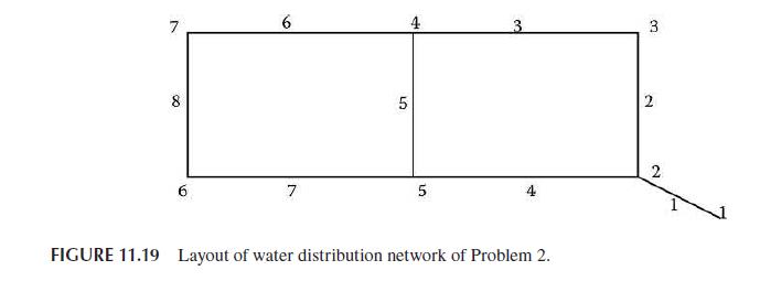
Calculate the system reliability of the water distribution network of Figure 11. 19 using the state enumeration method. Node 1 is the source node and other nodes are demand nodes.All of the pipes have the same failure probability equal to 5%. System reliability is defined as the ability of the
Calculate the reliability of the network of Problem 2 using cut-set analysis.Data from problem 2 Calculate the system reliability of the water distribution network of Figure 11. 19 using the state enumeration method. Node 1 is the source node and other nodes are demand nodes.All of the pipes have
Employ the tie-set analysis to calculate the reliability of water network described in Problem 2.Data from problem 2 Calculate the system reliability of the water distribution network of Figure 11. 19 using the state enumeration method. Node 1 is the source node and other nodes are demand nodes.All
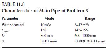
Determine the coefficient of variation of the loading and the capacity for a main pipe of a water distribution network with the parameters given in Table 11. 8. Consider a uniform distribution for definition of the uncertainty of each parameter. TABLE 11.8 Characteristics of Main Pipe of Problem 5
Using the results of Problem 5, determine the risk of the loading exceeding the capacity of the main pipe. Consider that MS = Qc − QL and MS follow the normal distribution.Data from problem 5 Determine the coefficient of variation of the loading and the capacity for a main pipe of a water
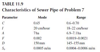
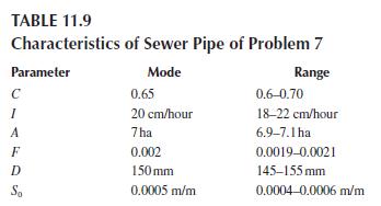
Determine the coefficient of variation of the loading and the capacity for a sewer pipe with the parameters given in Table 11. 9. The uncertainty of each parameter is defied with a triangular distribution. TABLE 11.9 Characteristics of Sewer Pipe of Problem 7 Parameter 1 Mode Range 0.65 0.6-0.70
Determine the risk of the loading exceeding the capacity of the sewer pipe in Problem 7.The MS is normally distributed and is calculated as MS = Qc/QL.Data from problem 7 Determine the coefficient of variation of the loading and the capacity for a sewer pipe with the parameters given in Table 11.
Apply the first-order analysis of uncertainty to the Darcy–Weisbach equation. Consider that S0,f, and d are uncertain.
Consider an 800-mm water transfer tunnel with mean loading equal to 2 m3/s and coefficient of variation equal to 0. 20. Calculate the risk of failure of a pipe using safety margin approach when MS is normally distributed. The energy slope of tunnel is 0. 0002 with a coefficient of variation of 0.
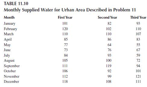
The monthly supplied water for an urban area in 3 years is presented in the Table 11. 10. The monthly mean water demand of the urban area is equal to 100 MCM. Evaluate the reliability, resiliency, and vulnerability of this urban water supply system for supplying more than 90% of urban water demand.
The concentration of a toxic chemical in an aquifer is 9. 8 mg/L. This aquifer is being used as the source of drinking water. Assume that the average weight of adult women in the area is 60 kg and they drink 1. 5 L of water per day, determine the total amount of the chemical that an adult woman may
Calculate the reliability of the water supply system shown in Figure 11. 19 at t = 0. 1 assuming that R(t)=R4 (t)=e-2 and R (t) = R(t) = R(t)=e,(1i2;1 j 3).
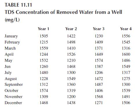
TDS concentration data of removed water from a well is presented in Table 11. 11. The standard value of TDS concentration in this region is considered as 1,400 (mg/L). Calculate the reliability, resiliency, and vulnerability of water quality requirement. TABLE 11.11 TDS Concentration of Removed
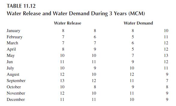
The monthly water withdrawals from an aquifer and monthly water demand during 3 years are presented in Table 11. 12. Calculate the reliability, resiliency, and vulnerability of this aquifer of water supply TABLE 11.12 Water Release and Water Demand During 3 Years (MCM) Water Demand 10 11 12 12 13
Appling the first-order analysis, formulate σQ and ΩQ in Manning’s equation [Q = (0.311/n)S1/2D8/3], where diameter D is a deterministic parameter and n and S are considered to be uncertain.
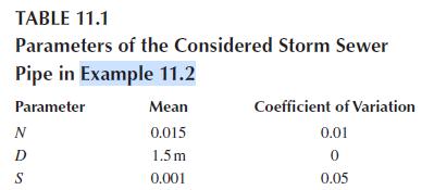
Determine the mean capacity of a storm sewer pipe, the coefficient of variation of the pipe capacity, and the standard deviation of the pipe capacity using Manning’s equation (refer to Example 11.1 ). The following parameter values can be considered as shown in Table 11.1 .Data from example 11.1
Evaluate the preparedness of the Tehran (capital of Iran) WDS. Because of the aging water distribution infrastructure of Tehran, the water pipe breaks are a common problem in this city. As there is not any rehabilitation program of aging pipes in this city, this problem is getting more severe over
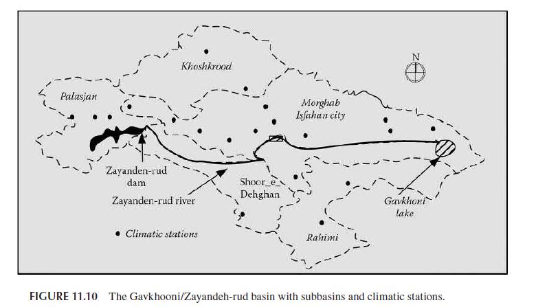
Evaluate the HDI for the Gavkhooni/Zayandeh-rud basin in central Iran. This basin has five subbasins with a total area of 41,347 km2. The dominant climate in this region is arid and semiarid. The precipitation varies throughout the basin between 2,300 mm in the west (where most of the precipitation
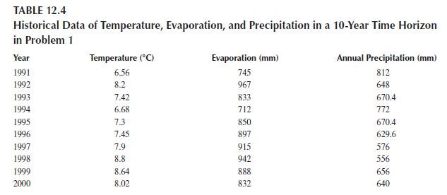
Assume that you want to model the rainfall–runoff of a basin in order to forecast the runoff in the coming years. The historical data of temperature, evaporation, and precipitation in a 10-year time horizon are presented in Table 12. 4. Formulate a multiple regression model for estimating the
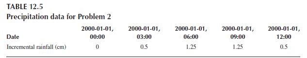
A 200 km2 watershed has a lag time of 100 minutes. Baseflow is considered constant at 20 cm. The watershed has a CN of 72% and 30% of imperviousness. Use HEC-HMS to determine the direct runoff for a storm using the SCS UH method. Precipitation data are presented in Table 12. 5. TABLE 12.5
An 8 km2 watershed has a time of concentration of 1. 0 hour. Use HEC-HMS to determine the direct runoff for a storm (rainfall hyetograph given in Table 12. 6) using the SCS UH method.a. You must create new basin, Meteorologic, and Control Specifications files either in the same project or in a new
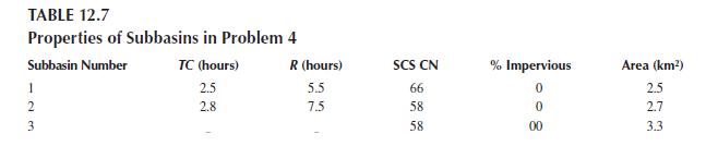
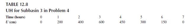
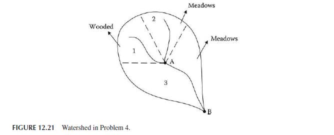
The parameters of a small undeveloped watershed are listed in Tables 12. 7 and 12. 8. A UH, and Muskingum routing coefficients are known for subbasin 3, as shown in Figure 12. 21.TC and R values for subbasins 1 and 2 and associated SCS CNs are provided as shown.A 5-hour rainfall hyetograph (in
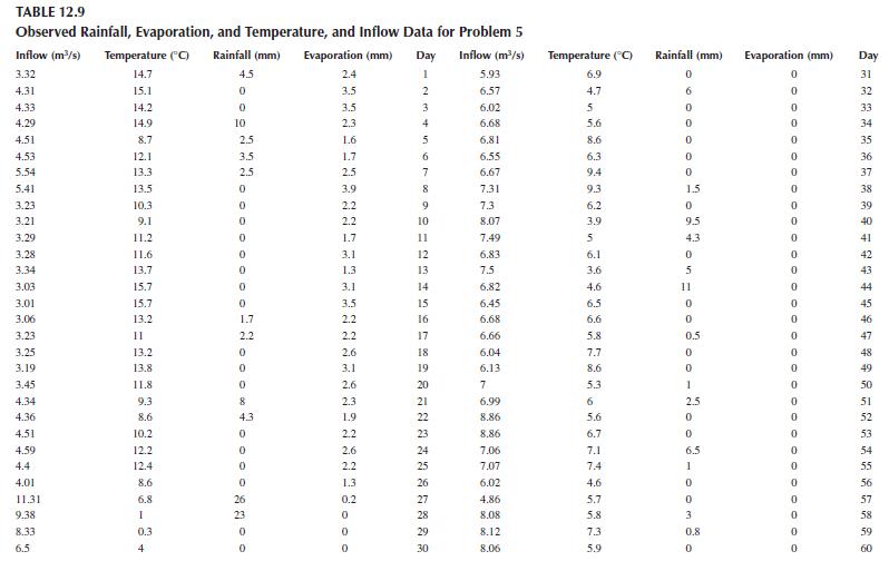
Develop an MLP model with two hidden layers and three perceptrons with logsig and linear function in each layer, respectively. The input of the MLP model is rainfall, evaporation, and temperature, and the inflow must be simulated. Use the given data in Table 12. 9 for model development. TABLE 12.9
Develop a TDL, GRNN, and RNN model for the data of Problem 5 and then compare and discuss the results of different simulations with ANN’s models.Data from problem 5 Develop an MLP model with two hidden layers and three perceptrons with logsig and linear function in each layer, respectively. The
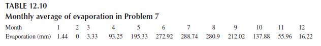
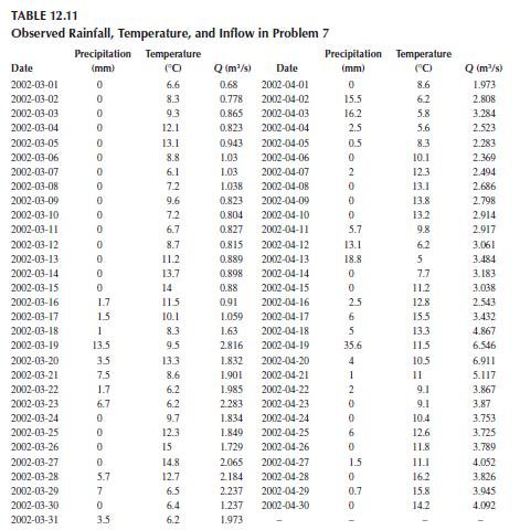
Calibrate the HBV model for the catchment described in Tables 12. 10 and 12. 11 for the period of March 1, 2002, to May 1, 2002. Discuss, before running the model, what effects you expect and then make a note of each change in parameter value and its effect on the simulation. TABLE 12.10 Monthly
Simulate the rainfall–runoff model in Problem 5 with IHACRES and then compare the difference between the next 2 months’ predictions with these two models.Data from problem 5 Develop an MLP model with two hidden layers and three perceptrons with logsig and linear function in each layer,
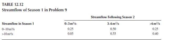
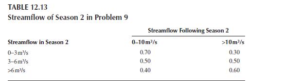
The transition probabilities of a Markov chain model for streamflow in two different seasons are given in Tables 12. 12 and 12. 13. Calculate the steady-state probabilities of flows in each interval in each season. TABLE 12.12 Streamflow of Season 1 in Problem 9 Streamflow in Season 1 0-10 m/s
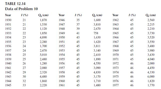
The data presented in Table 12. 14 is the annual maximum series (Qp) and the percentage of impervious area (I) for an urbanized watershed for the period from 1930 to 1977. Adjust the flood series to an eventual development of 50%. Estimate the effect on the estimated 2-, 10-, 25-, and 100-year
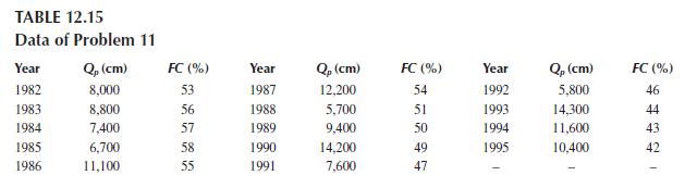
Residents in a community at the discharge point of a 614-km2 watershed believe that the recent increase in peak discharge rates is due to the deforestation by a logging company that has been occurring in recent years. Analyze the annual maximum discharges (Qp) and an average forest coverage (FC)
Analyze the data of Problem 5 to evaluate whether or not the increase in urbanization has been accompanied by an increase in the annual maximum discharge. Apply the Spearman test with both a 1% and a 5% level of significance. Discuss the results.Data from problem 5 Develop an MLP model with two
Consider two watersheds with different capacities for storage, such as sandy soil and clay with potential maximum retention of 7 and 5 cm, respectively, and also initial abstraction before ponding is 1. 5 cm. If a storm of 10 cm during 10 minutes occurs in both watersheds, determine the percentage

Showing 3100 - 3200 of 4723

First
25
26
27
28
29
30
31
32
33
34
35
36
37
38
39
Last

Step by Step Answers

Services

Sitemap
Fun
Definitions
Become Tutor
Used Textbooks
Study Help Categories
Recent Questions
Expert Questions
Campus Wear
Sell Your Books

Company Info

Security
Copyrights
Privacy Policy
Terms & Conditions
SolutionInn Fee
Scholarship
Online Quiz
Give Feedback, Get Rewards

Get In Touch

About Us
Contact Us
Career
Jobs
FAQ
Student Discount
Campus Ambassador

Secure Payment

Download Our App

© 2026 SolutionInn. All Rights Reserved