New Semester
Started
Get
50% OFF
Study Help!
--h --m --s
Claim Now
Question Answers
Textbooks
Find textbooks, questions and answers
Oops, something went wrong!
Change your search query and then try again
S
Books
FREE
Study Help
Expert Questions
Accounting
General Management
Mathematics
Finance
Organizational Behaviour
Law
Physics
Operating System
Management Leadership
Sociology
Programming
Marketing
Database
Computer Network
Economics
Textbooks Solutions
Accounting
Managerial Accounting
Management Leadership
Cost Accounting
Statistics
Business Law
Corporate Finance
Finance
Economics
Auditing
Tutors
Online Tutors
Find a Tutor
Hire a Tutor
Become a Tutor
AI Tutor
AI Study Planner
NEW
Sell Books
Search
Search
Sign In
Register
study help
mathematics
categorical data analysis
Categorical Data Analysis 2nd Edition Alan Agresti - Solutions
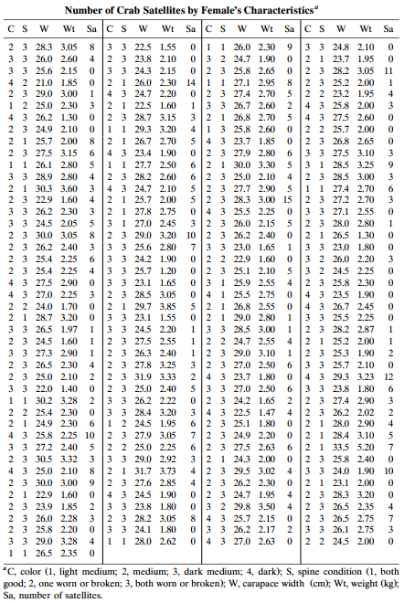
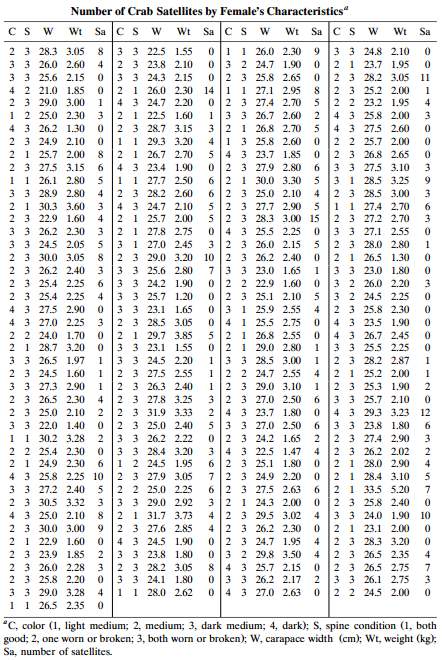
For Table 4.3, let Y = 1 if a crab has at least one satellite, and Y = 0 otherwise. Using x = weight, fit the linear probability model.a. Use ordinary least squares. Interpret the parameter estimates. Find the estimated probability at the highest observed weight (5.20 kg). Comment.b. Fit the
For Table 4.2, refit the linear probability model or the logistic regression model using the scores (a) (0, 2, 4, 6), (b) (0, 1, 2, 3), and (c) (1, 2, 3, 4). Compare β̂ for the three choices. Compare fitted values. Sum marize the effect of linear transformations of scores,
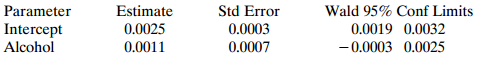
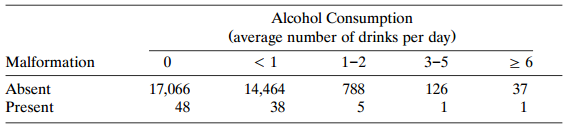
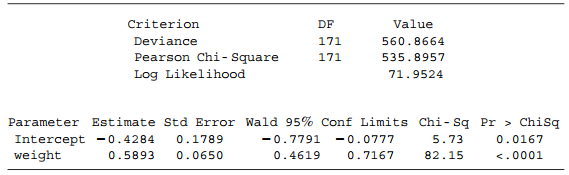
For Table 3.7 with scores (0, 0.5, 1.5, 4.0, 7.0) for alcohol consumption. ML fitting of the linear probability model for malformation has output.Interpret the model fit. Use it to estimate the relative risk of malformation for alcohol consumption levels 0 and 7.0.Table 3.7: Parameter Intercept
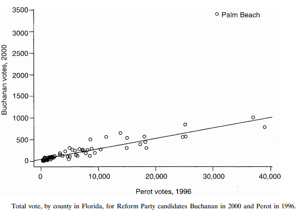
In the 2000 U.S. presidential election, Palm Beach County in Florida was the focus of unusual voting patterns (including a large number of illegal double votes) apparently caused by a confusing €œbutterfly ballot.€ Many voters claimed that they voted mistakenly for the Reform
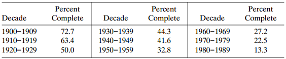
For games in baseball€™s National League during nine decades, Table 4.6 shows the percentage of times that the starting pitcher pitched a complete game.a. Treating the number of games as the same in each decade, the ML fit of the linear probability model is π̂ =
Refer to Problem 4.6. The sample mean and variance are 5.0 and 4.2 for treatment A and 9.0 and 8.4 for treatment B.a. Is there evidence of overdispersion for the Poisson model having a dummy variable for treatment? Explain.b. Fit the negative binomial loglinear model. Note that the estimated
For Table 4.3, Table 4.7 shows SAS output for a Poisson loglinear model fit using X = weight and Y = number of satellites.a. Estimate E(Y) for female crabs of average weight, 2.44 kg.b. Use β̂ to describe the weight effect. Show how to construct the reported confidence
Refer to Problem 4.7. Using the identity link with x = weight, µÌ‚ = €“2.60 + 2.264x, where β̂ = 2.264 has SE = 0.228. Repeat parts (a) through (c).Data from Prob. 4.7:For Table 4.3, Table 4.7 shows SAS output for a Poisson loglinear model fit
Refer to Table 4.3.a. Fit a Poisson loglinear model using both W = weight and C = color to predict Y = number of satellites. Assigning dummy variables, treat C as a nominal factor. Interpret parameter estimates.b. Estimate E(Y) for female crabs of average weight (2.44 kg) that are (i) medium light,
In Section 4.3.2, refer to the Poisson model with identity link. The fit using least squares is µ̂ = –10.42 + 0.51x (SE = 0.11). Explain why the parameter estimates differ and why the SE values are so different.
For the negative binomial model fitted to the crab satellite counts with log link and width predictor, µ̂ = –4.05, β̂ = 0.192 (SE = 0.048), k̂–1 = 1.106 (SE = 0.197). Interpret. Why is SE for β so different from SE = 0.020 for the corresponding Poisson GLM in Sec 4.3.2? Which is more
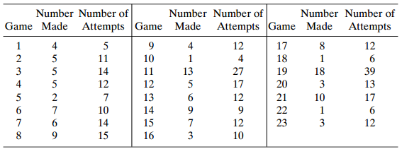
Table 4.8 shows the free-throw shooting, by game, of Shaq O€™NeaI of the Los Angeles Lakers during the 2000 NBA (basketball) playoffs. Commentators remarked that his shooting varied dramatically from game to game. In game i, suppose that Yi= number of free throws made out of niattempts is
Refer to Problem 4.6. The wafers are also classified by thickness of silicon coating (z = 0, low; z = 1, high). The first five imperfection counts reported for each treatment refer to z = 0 and the last five refer to z = 1. Analyze these data.Data from Prob. 4.6:An experiment analyzes imperfection
Describe the purpose of the link function of a GLM. What is the identity link? Explain why it is not often used with binomial or Poisson responses.
For binary data, define a GLM using the log link. Show that effects refer to the relative risk. Why do you think this link is not often used?
For the logistic regression model with 3 > 0, show that (a) as x → ∞, π(x) is monotone increasing, and (b) the curve for π(x) is the cdf of a logistic distribution having mean – α/β and standard deviation π/(|β|√3/).
Let Yi be a bin(ni, πi) variate for group i, i = 1, ...... N, with {Yi} independent. Consider the model that π1 = .... = πN. Denote that common value by π. For observations {yi} show that π̂ = (∑yi)/(∑ni).When all ni = 1, for testing this model’s fit in the N × 2 table, show that X2 =
A binomial GLM πi = Φ(∑j βj xij) with arbitrary inverse link function Φ assumes that niYi has a bin(ni, πi) distribution. Find wi in (4.27) and hence cov͡ (β̂). For logistic regression, show that wi = ni πi(1 – πi).
A GLM has parameter β with sufficient statistic S. A goodness-of-fit test statistic T has observed value to. If β were known, a P-value is P = P(T ≥ to; β). Explain why P(T ≥ to | S) is the uniform minimum variance unbiased estimator of P.
Let yij be observation j of a count variable for group i, i = 1,...,I, j = 1,..., ni. Suppose that {Yij} ae independent Poisson with E(Yij) = µi.a. Show that the ML estimate of µi is µ̂i = y̅i = ∑j yij/ni,b. Simplify the expression for the deviance for this model. [For testing this model, it
Consider the class of binary models (4.8) and (4.9). Suppose that the standard cdf Φ corresponds to a probability density function ϕ that is symmetric around 0.a. Show that x at which π(x) = 0.5 is x = – α/β.b. Show that the rate of change in π(x) when π(x) = 0.5 is βϕ(0).Show this is
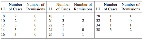
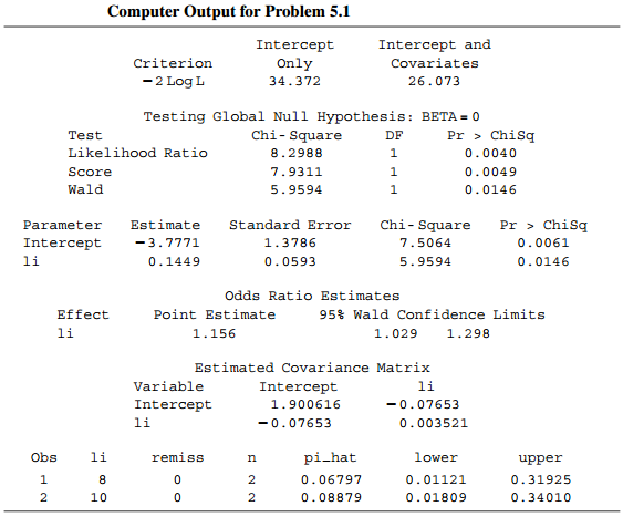
For a study using logistic regression to determine characteristics associated with remission in cancer patients, Table 5.10 shows the most important explanatory variable, a labeling index (U). This index measures proliferative activity of cells after a patient receives an injection of tritiated
According to the Independent newspaper (London, Mar. 8, 1994), the Metropolitan Police in London reported 30,475 people as missing in the year ending March 1993. For those of age 13 or less, 33 of 3271 missing males and 38 of 2486 missing females were still missing a year later. For ages 14 to 18,
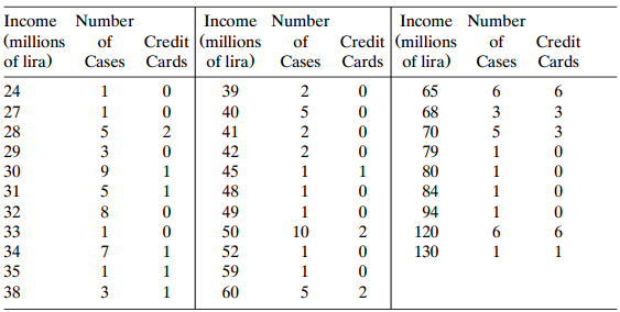
Table 5.19 refers to a sample of subjects randomly selected for an Italian study on the relation between income and whether one possesses a travel credit card. At each level of annual income in millions of lira, the table indicates the number of subjects sampled and the number possessing at least
For the population of subjects having Y = j, X has a N(µj, σ2)distribution, j = 0,1.Using Bayes theorem, show that P(Y = 1|x) satisfies the logistic regression model with β = (µ1 – µ0))/σ2.
For an I × 2 contingency table, consider logit model (5.4).Given (πi > 0), show how to find (βi) satisfying βI = 0.
Let Yibe bin(ni, Ï€i) at xi, and let pi= yi/ni. For binomial GLMs with logit link:a. For pi near Ï€i, show thatb. Show that z1(t) in (5.23) is a linearized version of the ith sample logit, evaluated at approximation Ï€i(t) for π̂i. Pi – Ti Pi
Using graphs or tables, explain what is meant by no interaction in modeling response Y and explanatory X and Z when:a. All variables are continuous (multiple regression).b. Y and X are continuous, Z is categorical (analysis of covariance).c. Y is continuous, X and Z are categorical (two-way
Show that the conditional ML estimate of θ satisfies n211 = E(n11) for distribution (3.18).
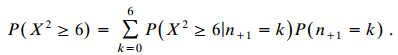
A Monte Carlo scheme randomly samples M separate I × J tables having observed margins to approximate Po = P(X2 ≥ X2o) for an exact test. Let P̂ be the sample proportion of the M tables with X2 ≥ X2o. Show that P(|P̂ – Po| ≤ B) = 1 – α requires that M ≈ z2α/2 Po(1–Po)/B2.
Consider exact tests of independence, given the marginais, for the I × I table having nii = 1 for i = 1,.....I, and nij = 0 otherwise.Show that (a) tests that order tables by their probabilities, X2, or G2 have P-value = 1.0, and (b) the one-sided test that orders tables by an ordinal statistic
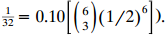
Refer to Problem 3.42 and exact tests using X2with Hα: Ï€1‰ Ï€2. Explain why the unconditional P-value, evaluated at Ï€ = 0.5, is related to Fisher conditional P-values for various tables by Thus, the unconditional P-value of 1/32 is a
A contingency table for two independent binomial variable has counts (3, 0 / 0, 3) by row. For H0: π1 = π2 and Hα : π1 > π2, show that the P-value equals 1/64 for the exact unconditional test and 1/20 for Fisher’s exact test.
When a test statistic has a continuous distribution, the P-value has a null uniform distribution, P(P-value ≤ α) = α for 0 < α < 1. For Fisher’s exact test, explain why under the null, P(P-value ≤ α) ≤ α for 0 < α < 1.
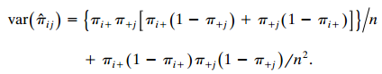
Assume independence, and let pij= nij/n and π̂ij= pi+p+j.a. Show that pij and π̂ij are unbiased for Ï€ij = Ï€i+ Ï€+j.b. Show that var(pij) = Ï€i+ Ï€+j(1 €“ Ï€i+
Use a partitioning argument to explain why G2 for testing independence cannot increase after combining two rows (or two columns) of a contingency table.
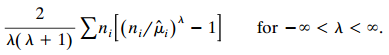
For counts {ni}, the power divergence statistic for testing goodness of fit is
For testing independence, show that X2 ≤ n min (I – 1, J – 1). Hence V2 = X2 / [n min(I – 1, J – 1)] falls between 0 and 1 (Carmer 1946). For 2 × 2 tables, X2 / n is often called phi-squared; it equals Goodman and Kruskal’s tau. Other measures based on X2 include the contingency
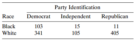
Refer to Table 3.10. a. Using X2 and G2, test the hypothesis of independence between party identification and race. Report the P-values and interpret.b. Partition chi-squared into components regarding the choice between Democrat and Independent and between these two combined and Republican.
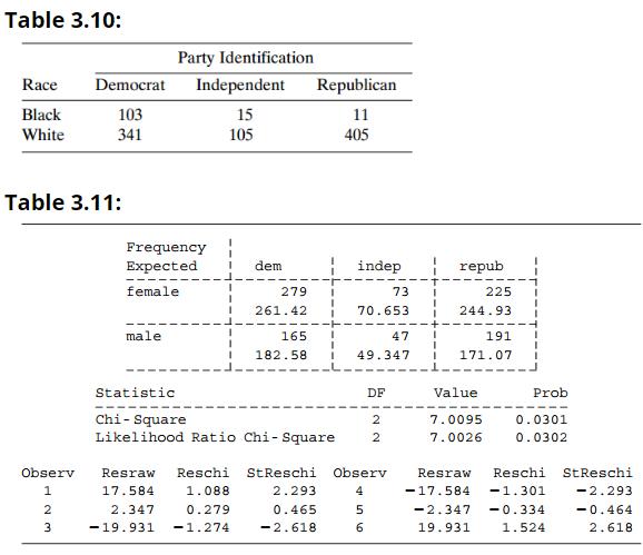
Refer to Table 3.10. In the same survey, gender was cross-classified with party identification. Table 3.11 shows some results. Explain how to interpret all the results on this printout. Table 3.10: Party Identification Race Democrat Independent Republican Black 103 341 15 11 White 105 405 Table
In a study of the relationship between stage of breast cancer at diagnosis (local or advanced) and a woman’s living arrangement, of 144 women living alone, 41.0% had an advanced case; of 209 living with spouse, 52.2% were advanced; of 89 living with others, 59.6% were advanced. The authors
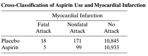
Refer to Table 2.1. Partition G2for testing whether the incidence of heart attacks is independent of aspirin intake into two components. Interpret.Table 2.1: Cross-Classification of Aspirin Use and Myocardial Infarction Myocardial Infarction Fatal Nonfatal No Attack Attack Attack Placebo 18 171
Project Blue Book: Analysis of Reports of Unidentified Aerial Objects was published by the U.S. Air Force (Air Technical Intelligence Center at Wright-Patterson Air Force Base) ¡n May 1955 to analyze reports of unidentified flying objects (UFOs). In its Table II, the report classified 1765
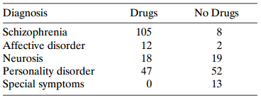
Table 3.12 classifies a sample of psychiatric patients by their diagnosis and by whether their treatment prescribed drugs.Partition chi-squared into three components to describe differences and similarities among the diagnoses, by comparing (I) the first two rows, (ii) the third and fourth rows,
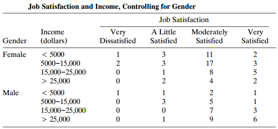
Refer to Table 7.8. For the combined data for the two genders, yielding a single 4 × 4 table, X2= 11.5 (P = 0.24), whereas using row scores (3, 10, 20, 35) and column scores (1, 3, 4, 5), M2= 7.04 (P = 0.008). Explain why the results are so different.Table 7.8: Job Satisfaction and
A study on educational aspirations of high school students (S. Crysdale, Internat. J. compar. Sociol. 16: 19–36, 1975) measured aspirations with the scale (some high school, high school graduate, some college, college graduate). The student counts in these categories were (11, 52, 23, 22) when
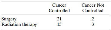
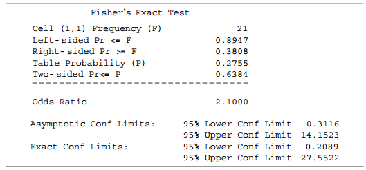
Table 3.13 shows the results of a retrospective study comparing radiation therapy with surgery in treating cancer of the larynx. The response indicates whether the cancer was controlled for at least two years following treatment. Table 3.14 shows SAS output.a. Report and interpret the P-value for
A study considered the effect of prednisolone on severe hypercalcaemia in women with metastatic breast cancer (B. Kristensen et al., J. Intern. Med. 232: 237–245, 1992). Of 30 patients, 15 were randomly selected to receive prednisolone. The other 15 formed a control group. Normalization in their
Consider a 3 × 3 table having entries, by row, of (4, 2, 0 / 2, 2, 2 / 0, 2, 4). Conduct an exact test of independence, using X2. Assuming ordered rows and columns and using equally spaced scores, conduct an ordinal exact test. Explain why results differ so much.
An advertisement by Schering Corp. in 1999 for the allergy drug Claritin mentioned that in a pediatric randomized clinical trial, symptoms of nervousness were shown by 4 of 188 patients on loratadine (Claritin), 2 of 262 patients taking placebo, and 2 of 170 patients on choropheniramine. In each
Is θ̂ the midpoint of large- and small-sample confidence intervals for θ? Why or why not?
For comparing two binomial samples, show that the standard error (3.1) of a log odds ratio increases as the absolute difference of proportions of successes and failures for a given sample increases.
Using the delta method, show that the Wald confidence interval for the logit of a binomial parameter π is log [π̂/(1–π̂)] ± zα/2/√nπ̂(1–π̂). Explain how to use this interval to obtain one for π itself. [Newcombe (2001) noted that the sample logit is also the midpoint of the score
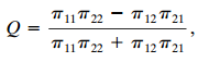
For multinomial sampling, use the asymptotic variance of log θ̂ to show that for Yule€™s Q the asymptotic variance of
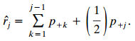
An I × J table has ordered columns and unordered rows. Ridits (Bross 1958) are data-based column scores. The jth sample ridit is the average cumulative proportion within category j,The sample mean ridit in row i is RÌ‚i = ˆ‘j rÌ‚j pj|i. Show that =
Show that X2 = n∑∑(pij – pi+ p+j)2/pi+ p+j. Thus, X2 can be large when n is large, regardless of whether the association is practically important. Explain why this test, like other tests, simply indicates the degree of evidence against H0 and does not describe strength of association.
For a 2 × 2 table, consider H0: π11 = θ2, π12 = π21 = θ(1 – θ), π22 = (1 – θ)2.a. Show that the marginal distributions are identical and that independence holds.b. For a multinomial sample, under H0 show that θ̂ = (p1+ + p+1)/2.c. Explain how to test H0. Show that df = 2 for the test
The measure of association lambda for nominal variables (Goodman and Kruskal 1954) has V(Y) = 1 –max{π+j} and V(Y|i) = 1 – rnaxj{πj|i}. Interpret lambda as a proportional reduction in prediction error for predictions which select the response category that is most likely. Show that
When X and Y are ordinal with counts {nij}:a. Explain why the (n 2) pairs of observations partition into C + D + TX + TY €“ TXY, where TX = ˆ‘ni + (ni+ €“1)/2 pairs are tied on X, TY pairs are tied on Y, and TXY pairs are tied on X and Y.b. Explain why d is
For 2 × 2 tables, Yule (1900, 1912) introducedwhich he labeled Q in honor of the Belgian statistician Quetelet. It is now called Yule€™s Q.a. Show that for 2 × 2 tables, Goodman and Kruskal€™s γ = Q.b. Show that Q falls between €“
Suppose that {Yij} are independent Poisson variates with means {µij}. Show that P(Yij = nij) for all i, j, conditional on {Yi+ = ni}, satisfy independent multinomial sampling [i.e., the product of (2.2) for all i] within the rows.
When X and Y are conditionally dependent at each level of Z yet marginally independent, Z is called a suppressor variable. Specify joint probabilities for a 2 × 2 × 2 table to show that this can happen (a) When there is homogeneous association, (b) When the association has opposite
Smith and Jones are baseball players. Smith has a higher batting average than Jones in each of K years. Is it possible that for the combined data from the K years, Jones has the higher batting average? Explain, using an example to illustrate.
For a 2 × 2 × 2 table, show that homogeneous association is a symmetric property, by showing that equal XY conditional odds ratios is equivalent to equal YZ conditional odds ratios.
Let πij|k = P(X = i, Y = j|Z = k). Explain why XY conditional independence is πij|k = πi+|k π+j|k for all i and j and k.
Explain why for three events E1, E2 and E3 and their complements, it is possible that P(E1 | E2) > P(E1 | E̅2) even if both P(E1 | E2 E3) < P(E1 | E̅2 E3) and P(E1 |E2 E̅3) < P(E1 |E̅2, E̅3).
For given π1 and π2 show that the relative risk cannot be farther than the odds ratio from their independence value of 1.0.
Let D denote having a certain disease and E denote having exposure to a certain risk factor. The attributable risk (AR) is the proportion of disease cases attributable to that exposure.a. Let P(E̅) = 1 – P(E). Explain why AR= [P(D) –P(D|E̅)]/P(D).b. Show that AR relates to the relative risk
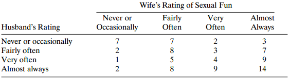
Table 2.12 summarizes responses of 91 married couples in Arizona to a question about how often sex is fun. Find and interpret a measure of association between wife€™s response and husband€™s response.Table 2.12: Wife's Rating of Sexual Fun Fairly Often Never or Almost Always
A study of the death penalty for cases in Kentucky between 1976 and 1991 (T. Keil and G. Vito, Amer. J. Criminal Justice 20: 17—36, 1995) indicated that the defendant received the death penalty in 8% of the 391 cases in which a white killed a white, in 2% of the 108 cases in which a black killed
At each age level, the death rate is higher in South Carolina than in Maine, but overall, the death rate is higher in Maine. Explain how this could be possible.
Based on 1987 murder rates in the United States, an Associated Press story reported that the probability that a newborn child has of eventually being a murder victim is 0.0263 for nonwhite males, 0.0049 for white males. 0.0072 for nonwhite females, and 0.0023 for white females.a. Find the
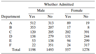
Table 2.10 refers to applicants to graduate school at the University of California at Berkeley, for fall 1973. It presents admissions decisions by gender of applicant for the six largest graduate departments. Denote the three variables by A = whether admitted, G = gender, and D = department. Find
A 20-year cohort study of British male physicians (R. Doll and R. Peto, British Med. J. 2: 1525–1536, 1976) noted that the proportion per year who died from lung cancer was 0.00140 for cigarette smokers and 0.00010 for nonsmokers. The proportion who died from coronary heart disease was 0.00669
A research study estimated that under a certain condition, the probability that a subject would be referred for heart catheterization was 0.906 for whites and 0.847 for blacks.a. A press release about the study stated that the odds of referral for cardiac catheterization for blacks are 60% of the
In an article about crime in the United States, Newsweek (Jan. 10, 1994) quoted FBI statistics for 1992 stating that of blacks slain, 94% were slain by blacks, and of whites slain, 83% were slain by whites. Let Y = race of victim and X = race of murderer. Which conditional distribution do these
For adults who sailed on the Titanic on its fateful voyage, the odds ratio between gender (female, male) and survival (yes, no) was 11.4. a. What is wrong with the interpretation. “The probability of survival for females was 11.4 times that for males”? Give the correct interpretation. When
In the United States, the estimated annual probability that a woman over the age of 35 dies of lung cancer equals 0.001304 for current smokers and 0.000121 for nonsmokers (M. Pagano and K. Gauvreau, Principles of Biostatistics, Duxbury Press, Pacific Grove, CA. 1993, p. 134).a. Find and interpret
A newspaper article preceding the 1994 World Cup semifinal match between Italy and Bulgaria stated that “Italy is favored 10–11 to beat Bulgaria, which is rated at 10–3 to reach the final.” Suppose that this means that the odds that Italy wins are 11/10 and the odds that Bulgaria wins are
A study (E. G. Krug et al., Internat. J. Epiderniol., 27: 214-221, 1998) reported that the number of gun-related deaths per 100,000 people in 1994 was 14.24 in the United States, 4.31 in Canada, 2.65 in Australia, 1.24 in Germany, and 0.41 in England and Wales. Use the relative risk to compare the
Consider the following two studies reported in the New York Times.a. A British study reported (Dec. 3, 1998) that of smokers who get lung cancer, “women were 1.7 times more vulnerable than men to get small-cell lung cancer.” Is 1.7 the odds ratio or the relative risk?b. A National Cancer
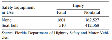
Table 2.9 is based on records of accidents in 1988 compiled by the Department of Highway Safety and Motor Vehicles in Florida. Identify the response variable, and find and interpret the difference of proportions, relative risk, and odds ratio. Why are the relative risk and odds ratio approximately
A diagnostic test has sensitivity = specificity = 0.80. Find the odds ratio between true disease status and the diagnostic test result.
An article in the New York Times (Feb. 17, 1999) about the PSA blood test for detecting prostate cancer stated: ‘The test fails to detect prostate cancer in 1 in 4 men who have the disease (false-negative results), and as many as two-thirds of the men tested receive false-positive results.” Let
The chi-squared mgf with df = ν is m(t) = (1–2t)–ν/2, for |t| < ½. Use it to prove the reproductive property of the chi-squared distribution.
For testing H0: Ï€j= Ï€j0j = 1,. . . ,c, using sample multinomial proportions {π̂j}, the likelihood-ratio statistic (1.17) isShow that G2 ‰¥ 0, with equality if and only if π̂j = Ï€j0 for all j. (Apply
Refer to quadratic form (1.16).For the zs statistic (1.11), show that z2S = X2 for c = 2.
Genotypes AA, Aa, and aa occur with probabilities [θ2, 2θ(1 – θ), (1 – θ)2]. A multinomial sample of size n has frequencies (n1, n2, n3) of these three genotypes.a. Form the log likelihood. Show that θ̂ = (2n1 + n2)/(2n1 + 2n2 + 2n3).b. Show that –∂2L(θ)/∂θ2 = [(2n1 + n2)/θ2] +
For I × J contingency tables, explain why the variables are independent when the (I – 1) (J – 1) differences πj|i – πj|1 = 0, i = 1,......., I – 1, j = 1,........., J – 1.
A binomial sample of size n has y = 0 successes.a. Show that the confidence interval for π based on the likelihood function is [0.0, 1 – exp( –z2a/2/2n)]. For a = 0.05, use the expansion of an exponential function to show that this is approximately [0,2/n].b. For the score method, show that
Consider the 95% binomial score confidence interval for π. When y = 1, show that the lower limit is approximately 0.18/n; in fact, 0 < π < 0.18/n then falls in an interval only when y = 0. Argue that for large n and π just barely below 0.18/n or just barely above 1 – 0.18/n, the actual
Consider the Wald confidence interval for a binomial parameter π. Since it is degenerate when π̂ = 0 or 1, argue that for 0 < π < 1 the probability the interval covers π cannot exceed [1 –πn – (1–π)n]; hence, the infimum of the coverage probability over 0 < π < 1 equals 0,
For a flip of a coin, let π denote the probability of a head. An experiment tests H0: π = 0.5 against Ha: π ≠ 0.5, using n = 5 independent flips.a. Show that the true null probability of rejecting H1 at the 0.05 significance level is 0.0 for the exact binomial test and using the large-sample
For a binomial parameter π, show how the inversion process for constructing a confidence interval works with (a) The Wald test, (b) The score test.
A researcher routinely tests using a nominal P(type I error) = 0.05, rejecting H0 if the P-value ≤ 0.05. An exact test using test statistic T has null distribution P(T = 0) = 0.30, P(T = 1) = 0.62, and P(T = 2) = 0.08, where a higher T provides more evidence against the null.a. With the usual
Inference for Poisson parameters can often be based on connections with binomial and multinomial distributions. Show how to test H0: µ1 = µ2 for two populations based on independent Poisson counts (y1,y2), using a corresponding test about a binomial parameter π. How can one construct a
Assume that y1, y2,. .., yn are independent from a Poisson distribution.a. Obtain the likelihood function. Show that the ML estimator µ̂ = y̅.b. Construct a large-sample test statistic for H0: µ. = µ0 using (i) the Wald method, (ii) the score method, and (iii) the likelihood-ratio method.c.
A likelihood-ratio statistic equals to,. At the ML estimates, show that the data are exp(to/2) times more likely under Ha than under H0.
From Section 1.4.2 the midpoint π̴ of the score confidence interval for π is the sample proportion for an adjusted data set that adds z2a/2/2 observations of each type to the sample. This motivates an adjusted Wald interval,Show that the variance
For a statistic T with cdf F(t) and p(t) = P(T = t), the mid-distribution function is Fmid(t) = F(t) – 0.5 p(t) (Parzen 1997). Given T = t0, show that the mid-P-value equals 1 – F(t0). (It also satisfies E[Fmid(T)] = 0.5 and var[Fmid(T)] = (1/12){1 – E[p2(T)]}.)
Showing 400 - 500
of 540
1
2
3
4
5
6
Step by Step Answers