New Semester Started Get 50% OFF Study Help! --h --m --s Claim Now

Question Answers

Textbooks

Find textbooks, questions and answers

Oops, something went wrong!

Change your search query and then try again

Result Not Found

Books FREE
Study Help
Tutors
AI Study Planner NEW
Sell Books

Search
Sign In
Register

study help
mathematics
categorical data analysis

Categorical Data Analysis 2nd Edition Alan Agresti - Solutions

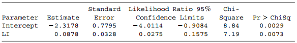
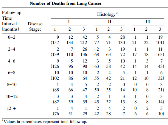
Consider Table 9.13. Explain how one could analyze whether the hazard depends on time.Table 9.13: Number of Deaths from Lung Cancer Follow-up Histology“ Time III I II Interval Disease (months) Stage: 2 3 3 2 0-2 12 42 5 4 28 1 19 (157 134 212 77 71 130 21 22 101) 2-4 2 26 2 3 19 11 (139 110 136
An article by W. A. Ray et al. (Amer. J. Epidemiol. 132: 873–884, 1992) dealt with motor vehicle accident rates for 16,262 subjects aged 65–84 years, with data on each for up to 4 years. In 17.3 thousand years of observation, the women had 175 accidents in which an injury occurred. In 21.4
A table at the text’s Web site (www.stat.ufl.edu/ ∼aa/cda/cda.html) shows the number of train miles (in millions) and the number of collisions involving British Rail passenger trains between 1970 and 1984. A Poisson model assuming a constant log rate α̂ over the 14-year period has α̂ =
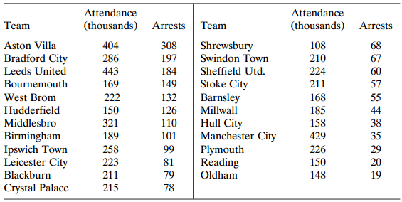
Table 9.18 lists total attendance (in thousands) and the total number of arrests in the 1987 €“ 1988 season for soccer teams in the Second Division of the British football league. Let Y = number of arrests for a team, and let t = total attendance. Explain why the model E(Y) = µt
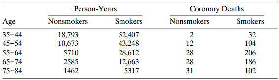
Table 9.19 is based on a study with British doctors.a. For each age, find the sample coronary death rates per 1000 person-years for nonsmokers and smokers. To compare them, take their ratio and describe its dependence on age.b. Fit a main-effects model for the log rates having four parameters for
In a 2 × 2 × K table, the true XY conditional odds ratios are identical, but different from the XY marginal odds ratio. Is there three-factor interaction? Is Z conditionally independent of X or Y? Explain.
Suppose that loglinear model (XY, XZ) holds.a. Find and log µij+. Show the loglinear model for the XY marginal table has the same association parameters as {λijXY} in (XY, XZ). Deduce that odds ratios are the same in the XY marginal table as in the partial tables. Using an analogous result for
For a four-way table, is the WX conditional association the same as the WX marginal association for the loglinear model (a) (WX, XYZ)? and (b) (WX, WZ, XY, YZ)? Why?
Loglinear model M0 is a special case of loglinear model M1.a. Haberman (1974a) showed that when {µ̂i} satisfy any model that is a special case of M0, ∑i µ̂1i log µ̂i = ∑i µ̂0i log µ̂i. Thus, µ̂0 is the orthogonal projection of µ̂1 onto the linear manifold of {log µ} satisfying
Consider the L × L model (9.6) with {υj = j} replaced by {υj = 2j}. Explain why β̂ is halved but {µ̂ij}, {θ̂ij}, and G2 are unchanged.
Lehmann (1966) defined (X, Y) to be positively likelihood-ratio dependent if their joint density satisfies f(x1, y1) f(x2, y2) ≥ f(x1, y2) f(x2, y1) whenever x1 < x2 and y1 < y2. Then, the conditional distribution of Y (X) stochastically increases as X (Y) increases.a. For the L × L model,
Yule (1906) defined a table to be isotropic if an ordering of rows and of columns exists such that the local log odds ratios are all nonnegative].a. Show that a table is isotropic if it satisfies (i) The linear-by-linear association model, (ii) The row effects model, and (iii) The RC
Consider the row effects model (9.8).a. Show that no loss of generality occurs in lettingb. Show that minimal sufficient statistics are {ni+}, {n+j}, and {ˆ‘j Ï…j nij, i = 1,..., I}, derive the likelihood equations. A = x} = µ, = 0. 0.
Refer to the homogeneous linear-by-linear association model (9.10).a. Show that the likelihood equations are, for all i, j, and k,b. Show that residual df = K(I €“ 1) (J €“ 1) €“ 1.c. When I = J = 2, explain why it is equivalent to (XY, XZ, YZ).d. Show how the last
When model (XY, XZ, YZ) is inadequate and variables are ordinal, useful models are nested between it and (XYZ). For ordered scores {ui}, {Ï…j} and {wk}, considera. Show that log odds ratios for any two variables change linearly across levels of the third variable.b. Show that the
Construct a model having general XZ and YZ associations, but row effects for the XY association that are (a) Homogeneous, and (b) Heterogeneous across levels of Z. Interpret.
Refer to Section 9.7.3. Let T = ∑ti and W = ∑wi. Suppose that survival times have a negative exponential distribution with parameter λ.a. Using log likelihood (9.19), show that λ̂ = W/T.b. Conditional on T, show that W has a Poisson distribution with mean Tλ. Using the Poisson likelihood,
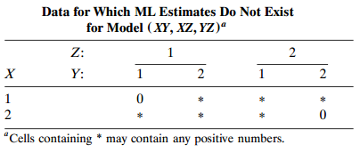
Show that ML estimates do not exist for Table 9.15. [Haberman: If µÌ‚111= c > 0, then marginal constraints the model satisfy imply that µÌ‚222= €“ c.]Table 9.15: Data for Which ML Estimates Do Not Exist for Model (XY, XZ, YZ)ª Z: 2 Y: 2 1 “Cells
For a loglinear model, explain heuristically why the ML estimate of a parameter is infinite when its sufficient statistics takes its maximum or minimum possible value, for given values of other sufficient statistics.
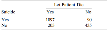
Table 10.14 shows results when subjects were asked €œDo you think a person has the right to end his or her own life if this person has an incurable disease?€ and When a person has a disease that cannot be cured, do you think doctors should be allowed to end the
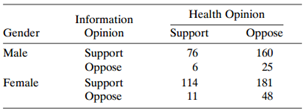
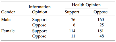
Refer to Table 8.16 and Problem 8.1. Treat the data as matched pairs on opinion, stratified by gender. Testing independence for the 2 Ã— 2 table using entries (6, 160) in row 1 and (11, 181) in row 2 tests equality of Î² for logit model (10.8) for each gender. Explain
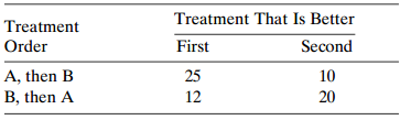
A crossover experiment with 100 subjects compares two drugs for treating migraine headaches. The response scale is success (1) or failure (0). Half the study subjects, randomly selected, used drug A the first time they had a headache and drug B the next time. For them, 6 had outcomes (1, 1) for (A,
A case–control study has 8 pairs of subjects. The cases have colon cancer, and the controls are matched with the cases on gender and age. A possible explanatory variable is the extent of red meat in a subject’s diet, measured as “1 = high” or “0 = low.” The (case, control) observations
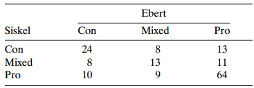
Each week Variety magazine summarizes reviews of new movies by critics in several cities. Each review is categorized as pro, con, or mixed, according to whether the overall evaluation is positive, negative, or a mixture of the two. Table 10.16 summarizes the ratings from April 1995 through
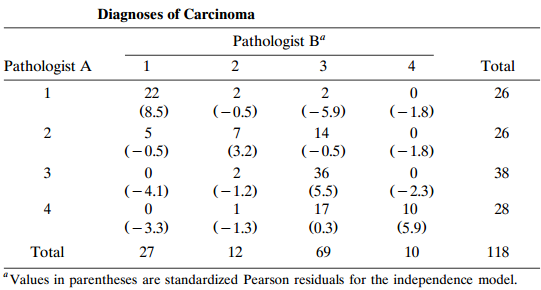
Refer to Table 10.8. Based on the reported standardized residuals, explain why the linear-by-linear association model (9.6) might fit well. Fit it and describe the association.Table 10.8: Diagnoses of Carcinoma Pathologist B“ Pathologist A 4 Total 1 22 26 1 (-5,9) (8.5) (-0.5) (–1.8) 5 14 26
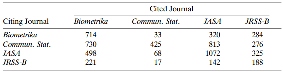
Table 10.20 refers to journal citations among four statistics journals during 1987 €“ 1989. The more often articles in a particular journal are cited, the more prestige that journal accrues. For citations involving pair A and B, view it as a victory for A if it is cited by B and a defeat
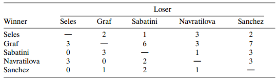
Table 10.21 refers to matches for several women tennis players during 1989 and 1990.a. Fit the Bradley€”Terry model. Interpret, and rank the players.b. Estimate the probability of Seles beating Graf. Compare the model estimate to the sample proportion. Construct a 90% confidence interval
Explain the following analogy: McNemar’s test is to binary data as the paired difference t test is to normally distributed data.
Refer to the subject-specific model (10.8) for binary matched pairs. a. Show that exp(Î²) is a conditional odds ratio between observation and outcome. Explain the distinction between it and the odds ratio exp(Î²) for model (10.6).b. For a random sample of n pairs, explain
Consider marginal model (10.6) when Y1 and Y2 are independent and conditional model (10.8) when {αi} are identical. Explain why they are equivalent.
Let Î²Ì‚M= log (p+1p2+/p+2p1+) refer to marginal model (10.6) and Î²Ì‚C= log (n21/n12) to conditional model (10.8). Using the delta method, show that the asymptotic variance of ˆšn(Î²Ì‚M€“ Î²M)
Give an example illustrating that when I > 2, marginal homogeneity does not imply symmetry.
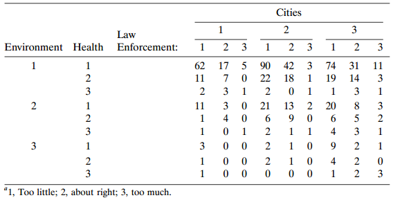
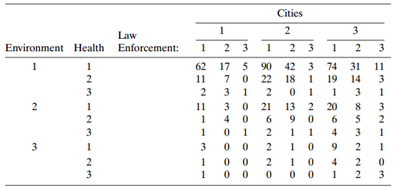
Refer to the 34table on government spending in Table 8.19. Analyze these data with a marginal cumulative logit model. Interpret effects.Table 8.19: Cities 2 3 1. Law Environment Health Enforcement: 3 3 2 3 62 17 5 90 42 3 74 31 11 2 22 18 19 14 3 11 3 2 3 2 3 3 21 13 20 8. 3 11 4 6. 2 1 3 2 4 3 3 3
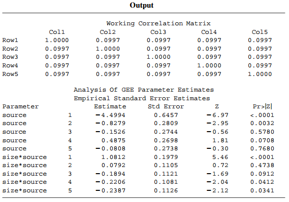
Refer to the air pollution data in Table 11.7. Using ML or GEE, fit marginal logit models that assume(a) Marginal homogeneity,(b) A linear effect of timeTable 11.7:
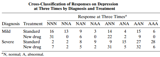
Refer to Table 11.2. Analyze the data using the scores (1, 2, 4) for the week number, using ML or GEE. Interpret estimates and compare substantive results to those in the text with scores (0, 1, 2).Table 11.2: Cross-Classification of Responses on Depression at Three Times by Diagnosis and Treatment
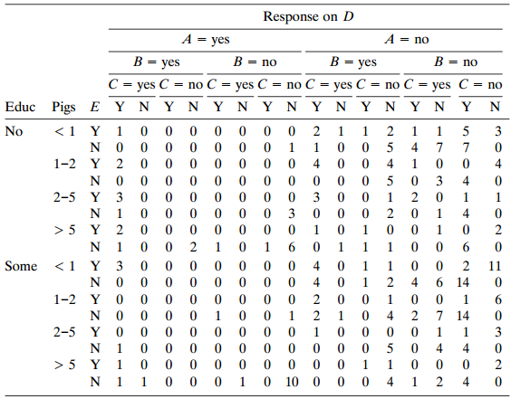
Table 11.11 is from a Kansas State University survey of 262 pig farmers. For the question €œWhat are your primary sources of veterinary information?,€ the categories were (A) professional consultant, (B) veterinarian, (C) state or local extension service, (D) magazines, and (E)
Refer to the matched-pairs data of Table 10.14 and Problem 10.1.a. Fit model (12.3). Interpret Î²Ì‚. If your software uses numerical integration, report Î²Ì‚, ÏƒÌ‚, and their standard errors for 5, 10, 25, 100, and 200 quadrature
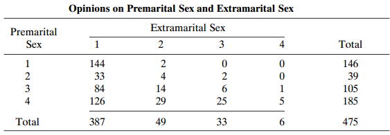
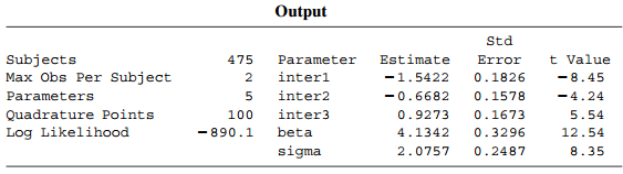
For marginal model (10.14) for Table 10.5 on premarital and extra marital sex, Table 12.12 shows results of fitting a corresponding random intercept model. Interpret Î²Ì‚. Compare estimates of and inferences about Î² to those in Section 10.3.2 for the marginal
For the insomnia example in Section 12.4.2, according to SAS the maximized log likelihood equals – 593.0, compared to – 621.0 for the simpler model forcing σ = 0. Compare models, using either a likelihood-ratio test or AIC. What do you conclude?
Refer to Section 12.3.1. Using supplementary information improves predictions. Let qi denote the true proportion of votes for Clinton in state i in the 1992 election, conditional on voting for him or Bush. Consider the modellogit[P(Yit = 1|ui)] = logit(qi) + α + ui,where {qi} are known and {ui}
For a binary response, consider the random effects modellogit[P(Yit = 1|ui)] = α + βt + ui, t = 1,..., T,where {ui} are independent N(0, σ2), and the marginal modellogit[P(Yt = 1)] = α + βt*, t = 1,..., T.For identifiability, βT = βT* = 0. Explain why all βt = 0 implies that all βt* = 0.
The GLMM for binary data using probit link function isΦ–1[P(Yit = 1 | ui)] = x’it β + z’it ui,where Φ is the N(0, 1) cdf and ui has N(0, ∑) pdf, f(ui; ∑).a. Show that the marginal mean isP(Yt = 1) = ʃ P(Z – z’it ui ≤ x’it β) f(ui; ∑) d ui,where Z is a standard normal
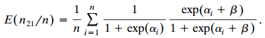
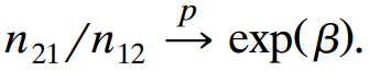
In the Rasch model, logit[P(Yit= 1)] = Î±i+ Î²t, Î±iis a fixed effect.a. Assuming independence of responses for different subjects and for different observations on the same subject, show that the log likelihood isb. Show that the likelihood equations are y+t =
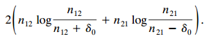
Consider the matched-pairs random effects model (12.3). For given Î²0, let Î´0be such that µÌ‚12= n12+ Î´0and µÌ‚21= n21€“ Î´0satisfies log(µÌ‚21/µÌ‚12) = Î²0.
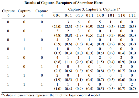
Explain why the logistic-normal model is not helpful for capture–recapture experiments with only two captures.
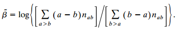
For ordinal square I Ã— I tables of counts {nab}, model (12.3) for binary matched-pairs responses (Yi1, Yi2) for subject i extends tologit[P(Yit ‰¤ j|ui)] = Î±j + Î²xt + uiwith {ui} independent N(0, Ïƒ2) variates and x1 = 0 and x2 = 1.a.
Summarize advantages and disadvantages of using a GLMM approach compared to a marginal model approach. Describe conditions under which parameter estimators are consistent for (a) marginal models using GEE, (b) marginal models using ML, (c) GLMM using PQL, and (d) GLMM using ML.
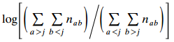
For capture €“ recapture experiments, Coull and Agresti (1999) used a loglinear model with exchangeable association and no higher-order terms. Explain why the model expected frequencies satisfylog µ(y1,..., yT) = Î» + Î²1 y1 + ... + Î²T yT +
A data set on pregnancy rates among girls under 18 years of age in 13 north central Florida counties has information on a 3-year total for each county i on ni = number of births and yi = number of those for which mother had age under 18.a. A beta-binomial model states that given {πi}, {Yi} are
In Problem 12.2 about Shaq O€™Neal€™s free-throw shooting, the simple binomial model, Ï€i= Î±, has lack of fit. Fit the beta-binomial model, or use the quasi-likelihood approach with that variance structure. Use the fit to summarize his free-throw
For the train accidents in Problem 9.19, a negative binomial model assuming constant log rate over the 14-year period has estimate –4.177 (SE = 0.153) and estimated dispersion parameter 0.012. Interpret.Data from Problem 9.19:A table at the text’s Web site
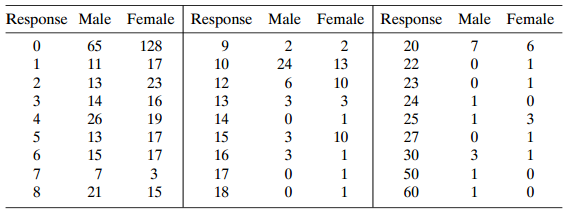
One question in the 1990 General Social Survey asked subjects how many times they had sexual intercourse in the preceding month. Table 13.9 shows responses, classified by gender.a. The sample means were 5.9 for males and 4.3 for females; the sample variances were 54.8 and 34.4. The mode for each
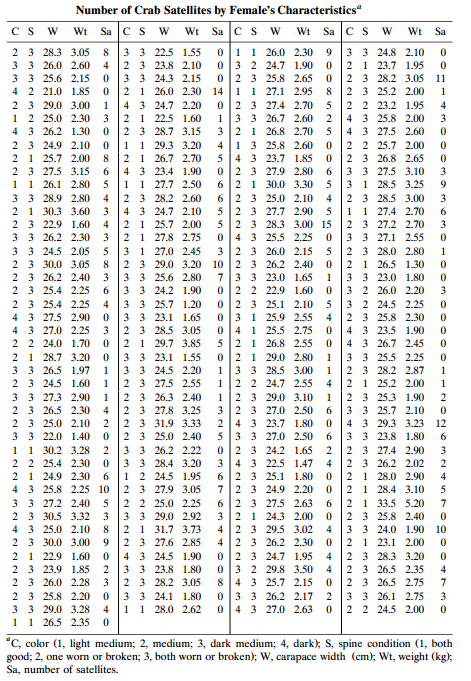
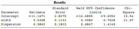
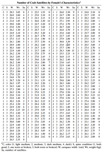
For the counts of horseshoe-crab satellites in Table 4.3, Table 13.10 shows the results of ML fitting of the negative binomial model using width as the predictor, with the identity link.a. State and interpret the prediction equation.b. Show that at a predicted µÌ‚, the estimated
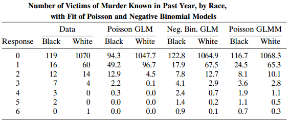
Refer to Table 13.6. For those with race classified as €œother,€ the sample counts for (0, 1, 2, 3, 4, 5, 6) homicides were (55, 5, 1, 0, 1, 0, 0). Fit an appropriate model simultaneously to these data and those for white and black race categories. Interpret by making pairwise
Let Y be a Poisson random variable with mean µ.a. For a constant c > 0, show thatE[log(Y + c)] = log µ + (c – 1/2)/µ + O(µ–2)(Note that log(Y + c) = log µ + log[1 + (Y + c – µ)/µ].)b. Cell counts in a 2 × 2 table are independent Poisson random variables. Use part (a) to argue that
Let p denote the sample proportion for n independent Bernoulli trials. Find the asymptotic distribution of the estimator [p(1 – p)]1/2 of the standard deviation. What happens when π = 0.5?
a. Refer to Problem 14.6. If Tn is Poisson, show √Tn has asymptotic variance 1/4.b. For a binomial sample with n trials and sample proportion p, show the asymptotic variance of sin-1(√p) is 1/4n. [This transformation and the one in part (a) are variance stabilizing, producing variates with
For a multinomial (n, {πi}) distribution, show the correlation between pi and pj is –[πi πj/(1 – πi)(1 – πj)]1/2. What does this equal when πi = 1 – πj and πk = 0 for k ≠ i, j?
Consider the model for a 2 × 2 table. π11 = θ2, π12 = π21 = θ(1 – θ), π22 = (1 – θ)2, where θ is unknown (Problems 3.31 and 10.34).a. Find the matrix A in (14.14) for this model.b. Use A to obtain the asymptotic variance of θ̂. (As a check, it is simple to find it directly using the
Suppose that {µij = nπij} satisfy the independence model (8.1).a. Show that λYa – λYb = log(π+a / π+b).b. Show that {all λYj = 0} is equivalent to π+j = 1/J for all j.
The book’s Web site (www.stat.ufl.edu/ ∼aa/cda/cda.html) has a 2 × 3 × 2 × 2 table relating responses on frequency of attending religious services, political views, opinion on making birth control available to teenagers, and opinion about a man and woman having sexual relations before
For a multiway contingency table, when is a logit model more appropriate than a loglinear model? When is a loglinear model more appropriate?
Refer to the logit model in Problem 5.24. Let A = opinion on abortion.a. Give the symbol for the loglinear model that is equivalent to this logit model.b. Which logit model corresponds to loglinear model (AR. AP, GRPY?c. State the equivalent loglinear and logit models for which (I) A is jointly
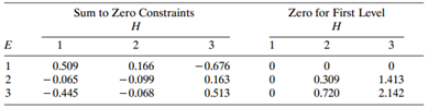
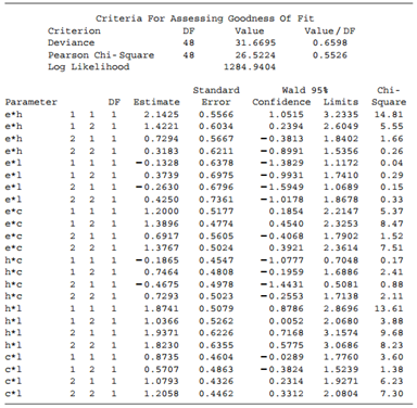
Refer to Table 8.19. Subjects were asked their opinions about government spending on the environment (E), health (H), assistance to big cities (C), and law enforcement (L).a. Table 8.20 shows some results, including the two-factor estimates, for the homogeneous association model. Check the fit, and
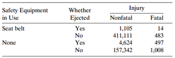
Table 8.18 refers to automobile accident records in Florida in 1988.a. Find a loglinear model that describes the data well. Interpret associations.b. Treating whether killed as the response, fit an equivalent logit model. Interpret the effects.Table 8.18: Safety Equipment in Use Seat belt Whether
Refer to Section 8.3.2. Explain why software for which parameters sum to zero across levels of each index reports λ̂11AC = λ̂22AC = 0.514 and λ̂12AC = λ̂21AC = – 0.514, with SE = 0.044 for each term.
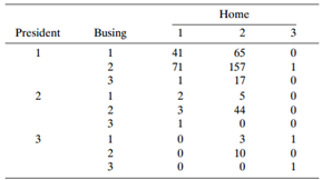
Refer to Table 8.17 from the 1991 General Social Survey. White subjects were asked: (B) €œDo you favor busing of (Negro/Black) and white school children from one school district to another?€, (P) €œIf your party nominated a (Negro/Black) for President, would you vote
The 1988 General Social Survey compiled by the National Opinion Research Center asked: €œDo you support or oppose the following measures to deal with AIDS9 (1) Have the government pay all of the health care costs of AIDS patients; (2) Develop a government information program to promote
For the multinomial (n,{Ï€j}) distribution with c > 2, confidence limits for Ï€jare the solutions of a. Using the Bonferroni inequality, argue that these c intervals simultaneously contain all {Ï€j} (for large samples) with probability at least 1€“ $| (गी, - मे) ° 2a/2 .{[i) + मै; - (मं) - मे.)}]/^}$
Refer to Section 1.5.6. Using the likelihood function to obtain the information, find the approximate standard error of π̂.
In some situations, X2 and G2 take very similar values. Explain the joint influence on this event of (a) whether the model holds, (b) whether the sample size n is large, and (c) whether the number of cells N is large.
Consider the logistic-normal model (12.10) for the abortion opinion data, under the constraint σ = 0.a. Explain why the fit is the same as an ordinary logit model treating the three responses for each subject as if they were independent responses for three separate subjects.b. Fit the model.
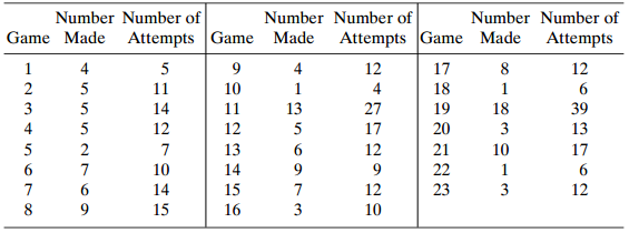
Refer to Table 4.8 on the free-throw shooting of Shaq O€™Neal. In game i, suppose that yi= number made out of niattempts is a bin(ni, Ï€i) variate and {yi} are independent.a. Fit the model, logit(Ï€i) = Î±. Find and interpret Ï€Ì‚i.
Gamblers A and B have a total of I dollars. They play games of pool repeatedly. Each game they each bet $1, and the winner takes the other’s dollar. The outcomes of the games are statistically independent, and A has probability π and B has probability 1 – π of winning any game. Play stops
Suppose that loglinear model (Y0, Y1,...,YT) holds. Is this a Markov chain?
What is wrong with this statement?: “For a first-order Markov chain, Yt is independent of Yt–2.”
a. For a univariate response, how is quasi-likelihood (QL) inference different from ML inference? When are they equivalent?b. Explain the sense in which GEE methodology is a multivariate version of QL.c. Summarize the advantages and disadvantages of the QL approach.d. Describe conditions under
Consider the model µi = β, i = 1,..., n, for independent Poisson observations. For β̂ = y̅, show that the model-based asymptotic variance estimate is y̅/n, whereas the robust estimate of the asymptotic variance is ∑i (yi – y̅)2/n2. Which would you expect to be better (a) if the Poisson
Repeat Problem 11.23 assuming that υ(µi) = σ2 when actually var(Yi) = µi.Data from Problem 11.23:Consider the model µi = β, i = 1, ..., n, assuming that υ(µi) = µi. Suppose that actually var(Yi) = µi2. Using the univariate version of GEE described in section 11.4, show that u(β) =
Consider the model µi = β, i = 1, ..., n, assuming that υ(µi) = µi. Suppose that actually var(Yi) = µi2. Using the univariate version of GEE described in section 11.4, show that u(β) = ∑i(yi – β)/β and β̂ = y̅. Show that V in (11.10) equals β/n, the actual asymptotic variance
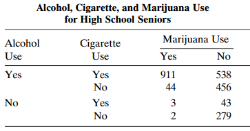
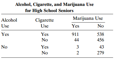
Refer to Problem 11.1. Suppose that we expressed the data with a 3 Ã— 2 partial table of drug-by-response for each subject, to use a generalized CMH procedure to test marginal homogeneity. Explain why the 911 + 279 subjects who make the same response for every drug have no effect on the
Refer to Problem 2.12.a. Fit the model with G and D main effects. Using it, estimate the AG conditional odds ratio. Compare to the marginal odds ratio, and explain why they are so different. Test its goodness of fit.b. Fit the two models excluding department A. Again consider lack of fit, and
For a sequence of s nested models M1,..., Ms, model Ms is the most complex. Let ν denote the difference in residual df between M1 and Ms.a. Explain why for j < k, G2(Mj | Mk) ≤ G2(Mj | Ms).b. Assume model Mj, so that Mk also holds when k > j. For all k > j, as n → ∞,
Prove that the Pearson residuals for the linear logit model applied to a I × 2 contingency table satisfy X2 = ∑1i = 1 e2i. Note that this holds for a binomial GL.M with any link.
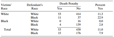
Refer to Table 2.6. Let D = defendant€™s race, V = victims€™ race, and P = death penalty verdict. Fit the loglinear model (DV, DP, PV).a. Using the fitted values, estimate and interpret the odds ratio between D and P at each level of V. Note the common odds ratio property.b.
For model (AC, AM, CM) with Table 8.3, the standardized Pearson residual in each cell equals ± 0.63. Interpret, and explain why each one has the same absolute value. By contrast, model (AM, CM) has standardized Pearson residual ± 3.70 in each cell where M = yes (e.g., + 3.70 when A =
Use odds ratios in Table 8.3 to illustrate the collapsibility conditions.a. For (A, C, M), all conditional odds ratios equal 1.0. Explain why all reported marginal odds ratios equal 1.0.b. For (AC, M), explain why (i) all conditional odds ratios are the same as the marginal odds ratios, and (ii)
Refer to Problem 5.1. Table 6.18 shows output for fitting a probit model. Interpret the parameter estimates (a) using characteristics of the normal cdf response curve, (b) finding the estimated rate of change in the probability of remission where it equals 0.5, and (c) finding the difference
The horseshoe crab width values in Table 4.3 have xÌ… = 26.3 and sx= 2.1. If the true relationship were similar to the fitted equation in Section 5.1.3, about how large a sample yields P(type II error) = 0.10, with Î± = 0.05, for testing H0: Î² = 0 against
For the horseshoe crab data, fit a model using weight and width as predictors. Conduct (a) A likelihood-ratio test of H0: β1 = β2, = 0, (b) Separate tests for the partial effects. Why does neither test in part (b) show evidence of an effect when the test in part (a) shows strong
Treatments A and B were compared on a binary response for 40 pairs of subjects matched on relevant covariates. For each pair, treatments were assigned to the subjects randomly. Twenty pairs of subjects made the same response for each treatment. Six pairs had a success for the subject receiving A
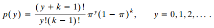
For a sequence of independent Bernoulli trials, Y is the number of successes before the kth failure. Explain why its probability mass function is the negative binomial,[For it, E(Y) = kÏ€/(1€“Ï€) and var(Y) = kÏ€/1(1€“Ï€)2, so var(Y) >
For the geometric distribution p(y) = πy(1– π), y = 0, 1, 2,... , show that the tail method for constructing a confidence interval [i.e., equating P(Y ≥ y) and P(Y ≤ y) to α/2] yields [(α/2)1/y, (1 – a/2)1/(y+1)]. Show that all π between 0 and 1 – a/2 never fall above a confidence
For a diagnostic test of a certain disease, π1 denotes the probability that the diagnosis is positive given that a subject has the disease, and π2 denotes the probability that the diagnosis is positive given that a subject does not have it. Let ρ denote the probability that a subject does have
For a 2 × 2 table of counts {nij} show that the odds ratio is invariant to(a) Interchanging rows with columns, (b) Multiplication of cell counts within rows or within columns by c ≠ 0. Show that the difference of proportions and the relative risk do not have these properties.
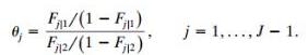
A 2 Ã— J table has ordinal response. Let Fj|i= Ï€1|i+ ..... + Ï€j|i. When Fj|2‰¤ Fj|1for j = 1,......, J, the conditional distribution in row 2 is stochastically higher than the one in row 1. Consider the cumulative odds ratios
For binary data with sample proportion yi based on ni trials, we use quasi-likelihood to fit a model using variance function. Show that parameter estimates are the same as for the binomial GLM but that the covariance matrix multiplies by ϕ.
Suppose that Yi is Poisson with g(µi) = a + βxi, where xi = 1 for i = 1,..., nA from group A and xi = 0 for i = nA + 1,..., nA + nB from group B. Show that for any link function g, the likelihood equations (4.22) imply that fitted means µ̂A and µ̂B equal the sample means.
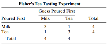
Refer to the tea-tasting data (Table 3.8). Construct the null distributions of the ordinary P-value and the mid-P-value for Fisher€™s exact test with HÎ±: 0 > 1. Find and compare their expected values.Table 3.8: Fisher's Tea Tasting Experiment Guess Poured First Poured
An experiment analyzes imperfection rates for two processes used to fabricate silicon wafers for computer chips. For treatment A applied to 10 wafers, the numbers of imperfections are 8, 7, 6, 6, 3, 4, 7, 2, 3, 4.Treatment B applied to 10 other wafers has 9,9,8, 14,8, 13, 11,5, 7,6 imperfections.

Showing 300 - 400 of 540

1
2
3
4
5
6

Step by Step Answers

Services

Sitemap
Fun
Definitions
Become Tutor
Used Textbooks
Study Help Categories
Recent Questions
Expert Questions
Campus Wear
Sell Your Books

Company Info

Security
Copyrights
Privacy Policy
Terms & Conditions
SolutionInn Fee
Scholarship
Online Quiz
Give Feedback, Get Rewards

Get In Touch

About Us
Contact Us
Career
Jobs
FAQ
Student Discount
Campus Ambassador

Secure Payment

Download Our App

© 2026 SolutionInn. All Rights Reserved