New Semester
Started
Get
50% OFF
Study Help!
--h --m --s
Claim Now
Question Answers
Textbooks
Find textbooks, questions and answers
Oops, something went wrong!
Change your search query and then try again
S
Books
FREE
Study Help
Expert Questions
Accounting
General Management
Mathematics
Finance
Organizational Behaviour
Law
Physics
Operating System
Management Leadership
Sociology
Programming
Marketing
Database
Computer Network
Economics
Textbooks Solutions
Accounting
Managerial Accounting
Management Leadership
Cost Accounting
Statistics
Business Law
Corporate Finance
Finance
Economics
Auditing
Tutors
Online Tutors
Find a Tutor
Hire a Tutor
Become a Tutor
AI Tutor
AI Study Planner
NEW
Sell Books
Search
Search
Sign In
Register
study help
mathematics
categorical data analysis
Categorical Data Analysis 2nd Edition Alan Agresti - Solutions
For Problem 3.14, obtain a 95% confidence interval for the odds ratio using(a) The Woolf (i.e., Wald) interval,(b) Cornfield’s ‘exact” approach, (c) the profile likelihood. In each case, note the effect of the zero cell count. Summarize advantages and disadvantages of each approach.Data from
For multinomial probabilities π = (π1, π2,......) with a contingency table of arbitrary dimensions, suppose that a measure g(π) = ν/δ. Show that the asymptotic variance of √n [g(π̂) – g(π)] is σ2 = [∑i πi η2i – (∑i πi ηi)2]/δ4, where ηi = δ(∂ν/∂πi) –
Let yi, i = 1,...,n, denote n independent binary random variables.a. Derive the log likelihood for the probit model Φ€“1 [Ï€(xi)] = ˆ‘j βj xij.b. Show that the likelihood equations for the logistic and probit regression models arewhere zi = 1
When J = 3, suppose that πj(x) = exp(αj + βjx)/[1 + exp(α1 + β1x) + exp(α2 + β2x)], j = 1, 2. Show that π3(x) is (a) decreasing in x if β1 > 0 and β > 0.
Suppose that model (7.24) holds for a 2 × J table with J > 2, and let x2 – x1 = 1. Explain why local log odds ratios are typically smaller in absolute value than the cumulative log odds ratio β. [McCullagh and Nelder (1989) noted that local odds ratios {θij} relate to β by logθij =
For the cumulative probit model Φ–1[P(Y ≤ j)] = αj – β’x, explain why a 1-unit increase in xi corresponds to a βi standard deviation increase in the expected underlying latent response, controlling for other predictors.
A cumulative link model for an I × J contingency table with a qualitative predictor is G–1[P(Y ≤ j)] = αj + µi, i = 1,...., I, j = 1,...., J – 1.a. Show that the residual df = (I – 1)(J – 2).b. When this model holds, show that independence corresponds to µ1 = ... = µI and the test of
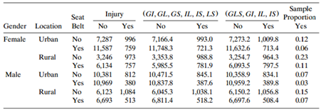
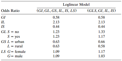
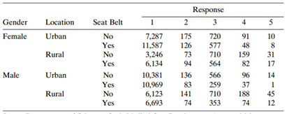
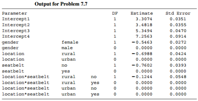
Refer to the loglinear models for Table 8.8.a. Explain why the fitted odds ratios in Table 8.10 for model (GI, GL, GS, IL, IS, LS) suggest that the most likely accident case for injury is females not wearing seat belts in rural locations.b. Fit model (GLS, GI, IL, IS). Using model parameter
For the loglinear model for an I × J table, log µij = λ + λiX, show that µ̂ij = ni+/J and residual df = I(J – 1).
Consider the loglinear model with symbol (XZ, YZ).a. For fixed k, show that {µ̂ijk} equal the fitted values for testing independence between X and Y within level k of Z.b. Show that the Pearson and likelihood-ratio statistics for testing this model’s fit have form X2 = ∑X2k, where X2k, tests
Consider loglinear model (X, Y, Z) for a 2 × 2 × 2 table.a. Express the model in the form log µ = Xβ.b. Show that the likelihood equations X’n = X’µ̂ equate {nijk} and {µ̂ijk} in the one-dimensional margins.
Given target row totals {ri > 0) and column totals {cj > 0):a. Explain how to use IPF to adjust sample proportions {pij} to have these totals but maintain the sample odds ratios.b. Show how to find cell proportions that have these totals and for which all local odds ratios equal θ > 0.
Consider loglinear model (WX, XY, YZ). Explain why W and Z are independent given X alone or given Y alone or given both X and Y. When are W and Y conditionally independent? When are X and Z conditionally independent?
Consider the log likelihood for the linear-by-linear association model.a. Differentiating with respect to β and evaluating at β = 0 and null estimates of parameters, show that the score function is proportional tob. Use the delta method to show that its null SE is ΣΣυν
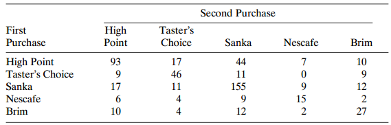
Table 10.17 shows subjects€™ purchase choice of instant decaffeinated coffee at two times.a. Fit the symmetry model and use residuals to analyze changes.b. Test marginal homogeneity. Show that the small P-value reflects a decrease in the proportion choosing High Point and an increase in
Calculate kappa for a 4 × 4 table having nii = 5 all i, ni, i+1 = 15, i = 1, 2, 3, n41 = 15, and nij = 0 otherwise. Explain why strong association does not imply strong agreement.
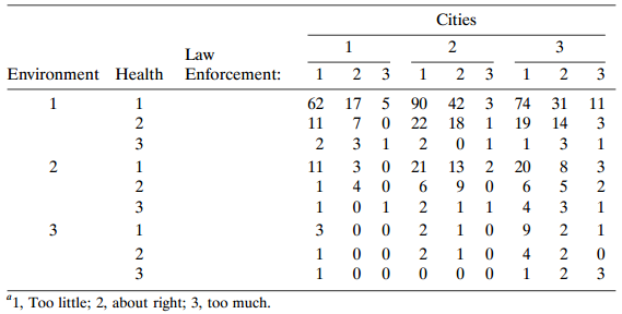
Refer to Table 8.19. The two-way table relating responses for the environment (as rows) and cities (as columns) has cell counts, by row, (108, 179, 157 / 21,55,52 / 5,6,24). Analyze these data.Table 8.19: Cities 2 3 1. Law Environment Health Enforcement: 3 3 2 3 62 17 5 90 42 3 74 31 11 2 22 18 19
Identify loglinear models that correspond to the logit models, for a < b, log(πab/πba) = (a) 0, (b) τ, (c) αa – αb, and (d) β(b – a).
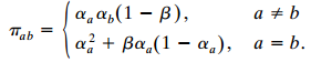
Consider the multiplicative model for a square table,a. Show that the model satisfies (i) symmetry, (ii) marginal homogeneity, (iii) quasi-symmetry, (iv) quasi-independence.b. Show that β = Cohen€™s kappa, and interpret K = 0 and K = 1 for this model. a + b a = b. a; + Ba„(1
A model for agreement on an ordinal response partitions beyond-chance agreement into that due to a baseline association and a main-diagonal increment. For ordered scores {ua}, the model isa. Show that this is a special case of quasi-symmetry and of quasi-association (10.29).b. Find the likelihood
Refer to the Bradley-Terry model.a. Show that log(Πac/Πca) = log(Πab/Πba) + log(Πbc/Πcb).b. With this model, is it possible that a could be preferred to b (i.e., Πab > Πba) and b could be preferred to c, yet c could be preferred to a? Explain.
Find the log likelihood for the Bradley–Terry model. From the kernel, show that (given {Nab}) the minimal sufficient statistics are {na+}. Thus, explain how “victory totals” determine the estimated ranking.
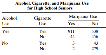
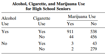
Refer to Table 8.3. Viewing the table as matched triplets, construct the marginal distribution for each substance. Find the sample proportions of students who used marijuana, alcohol, and cigarettes. Test the hypothesis of marginal homogeneity. Interpret results.Table 8.3: Alcohol, Cigarette, and
Refer to Problem 11.2. Further study shows evidence of an interaction between gender and substance type. Using GEE with exchangeable working correlation, the model fit for the probability Ï€ of using a particular substance islogit(π̂) = €“ 0.57 + 1.93S1 +
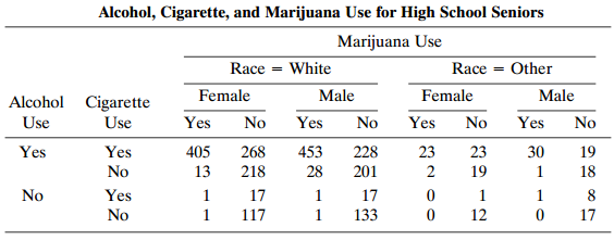
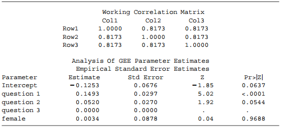
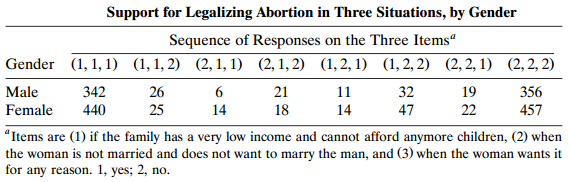
Refer to Table 11.13 on attitudes toward legalized abortion. For the response Yt(1 = support legalization, 0 = oppose) for question t (t = 1, 2, 3) and for gender g (1 = female, 0 = male), consider the model logit[P(Yt= 1)] = α + γg + βtwith β3=
Refer to Table 11.4.Fit the interaction modellogit[P(Y2 ‰¤ j)] = αj + β1x + β2 y1 + β3 xy1that constrains effects {β1x + β2 y1 + β3 xy1} to follow the pattern (Ï„, Ï„,
A first-order Markov chain has stationary (or time-homogeneous) transition probabilities if the one-step transition probability matrices are identical, that is, if for all i and j,πj|i(1) = πj|i(2) = ... = πj|i(T) = πj|i.Let X, Y, and Z denote the classifications for the I × I × T table
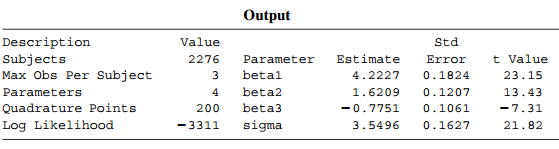
For table 8.3, let yit= 1 when subject i used substance t. Table 12.11 shows output for the logistic-normal modellogit[P(Yit = 1|ui)] = ui + βt.Interpret. Illustrate by comparing use of cigarettes and marijuana.Table 8.3:Table 12.11: Alcohol, Cigarette, and Marijuana Use for High School
How is the focus different for the model in Problem 12.3 than for the loglinear model (AC, AM, CM) used in Section 8.2.4? If σ̂ = 0, which loglinear model has the same fit as the GLMM?Data from Problem 12.3:For table 8.3, let yit = 1 when subject i used substance t. Table
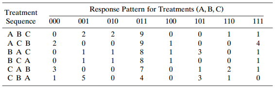
For the crossover study in Table 11.10 (Problem 11.6), fit the modellogit[P(Yi(k)t = 1|ui(k))] = αk + βt + ui(k),where {ui(k)} are independent N(0, σ2). Interpret {β̂t} and σ̂.Table 11.10: Response Pattern for
For Problem 12.7, fit the more general GLMM having treatment effects {βtk} that vary by sequence. Test whether the fit is better. One could also consider period or carryover effects. Add two period effects to model (12.19) (e.g., the first-period-effect parameter adds to the model when
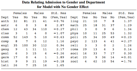
For Table 6.7 on admissions decisions for graduate school applicants, let yig= 1 denote a subject in department i of gender g (1 = females, 0 = males) being admitted.a. For the fixed effects model, logit[P(Yig = 1)] = α + βg + βiD, β̂ =
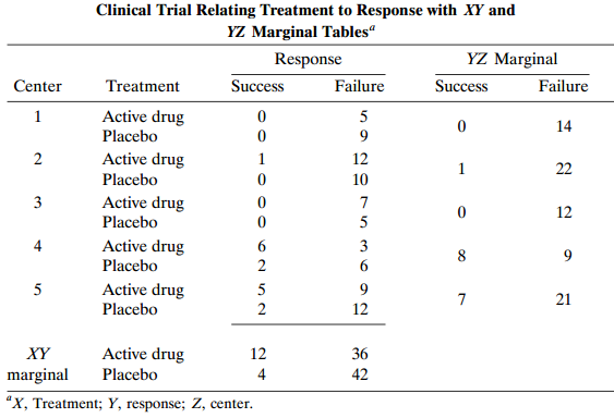
For the clinical trial in Table 9.16, let πit= P(Yit= 1 | ui) denote the probability of success for treatment t in center i.a. The random intercept model (12.11) has β̂ = 1.52 (SE = 0.70) and σ̂ = 1.9. Interpret.b. From Section 9.8.3, the
A data set from the 1994 General Social Survey on subjects’ opinions on four items (the environment, health, law enforcement, education) related to whether they believed government spending on each item should increase, stay the same, or decrease. Subjects were also classified by their gender and
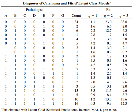
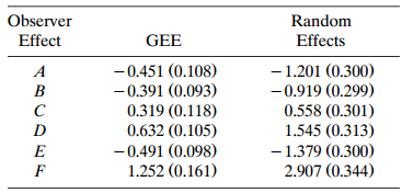
Landis and Koch (1977) showed ratings by seven pathologists who separately classified 118 slides regarding the presence and extent of carcinoma of the uterine cervix, using a five-point ordinal scale. For slide i with rater t, Table 12.14 shows results of fitting modellogit[P(Yit ‰¤
Refer to Section 12.5.1 on boys€™ attitudes toward the leading crowd. Table 12.15 shows results for a sample of schoolgirls. Fit model (12.16) and interpret. Summarize the estimated variability and correlation of random effects.Table 12.15:
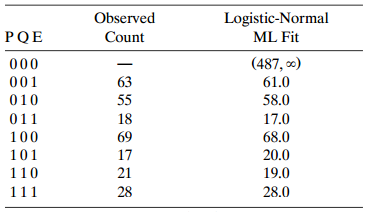
Table 12.16 reports results from a study to estimate the number N of people infected during a 1995 hepatitis A outbreak in Taiwan. The 271 observed cases were reported from records based on a serum test taken by the Institute of Preventive Medicine of Taiwan (P), records reported by the National
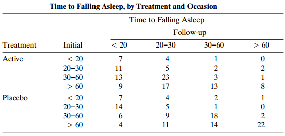
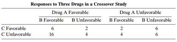
Analyze the crossover data of Table 11.1 using a random effects approach. Interpret, and compare results to those in Section 11.1.2.Table 11.1: Responses to Three Drugs in a Crossover Study Drug A Favorable B Unfavorable Drug A Unfavorable B Favorable B Unfavorable B Favorable C Favorable C
For the 23table of opinions about legalized abortion (Table 10.13) collapsed over gender, fit a latent class model with two classes. Show that it is saturated. For each latent class, report the estimated probability of supporting legalized abortion in each of the three situations. Give a tentative
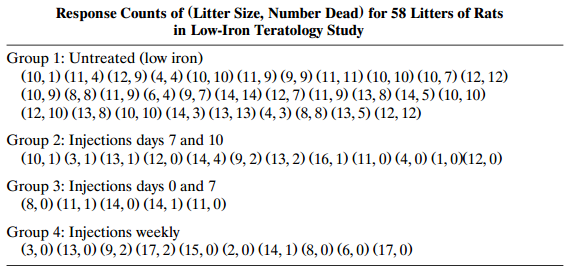
Extend the various analyses of the teratology data (Table 4.5) in Section 13.3.3 as follows:a. Include a predictor for litter size (as well as group). Interpret, and compare results to those without this predictor.b. Fit a model with beta-binomial variance (13.10) in which Ï varies by
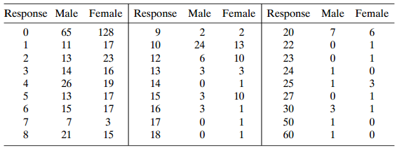
Refer to Problem 13.12. Fit the Poisson and negative binomial GLMs using identity link. Show that the estimated differences in means between males and females are identical for the two GLMs but the SE values are very different. Explain why. Use the more appropriate one to form a confidence interval
Derive residual df for a latent class model with q latent classes. When I = 2, for q ≥ 2 show one needs T ≥ 4 for the model to be unsaturated. Then, find the maximum value for q when T = 4, 5. For an I2 table, show one needs q < I2 /(2I – 1).
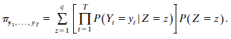
Express the log likelihood for latent class model (13.1) in terms of the model parameters. Derive likelihood equations. T Thy .. IIP(Y, = y,\Z = z) P(Z = z). 2=1 1=1
In Section 13.2.2, under the null that the ordinary logistic regression model holds, explain why ills inappropriate to treat the difference between the deviances for that model and the mixture of two logistic regressions as a chi-squared statistic.
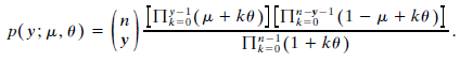
Show that the beta-binomial distribution (13.9) simplifies to the binomial when θ = 0. [Π3(μ + k0)] [Π3-(1-μ + k0)] Π3 (1+ kθ) p(y; μ, θ) - k=0
Suppose that Ï€i= P(Yit= 1) = 1 €“ P(Yit= 0), for t = 1,..., ni, and corr(Yit, Yis) = Ï for t ‰ s. Show that var(Yit) = Ï€i(1 €“ Ï€i), cov(Yit, Yis) = ÏÏ€i(1 €“ Ï€i), and ΣΥ-nτ,
When n = 1, show that the beta-binomial distribution is no different from the binomial (i.e., Bernoulli). Explain why overdispersion cannot occur when n = 1.
When y1,..., yNare independent from the negative binomial distribution (13.13) with k fixed, show that ?̂ = y̅. k Г(у + k) Г(k)Г(у + 1) etk k k p(y;k, µ) 1 u + k у %3D 0,1, 2, ....
Using E(Y) = E[E(Y | X)] and var(Y) = E[var(Y | X)] + var[E(Y | X)], derive the mean and variance of the(a) Beta-binomial distribution,(b) Negative binomial distribution.
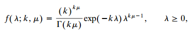
An alternative negative binomial parameterization results from the gamma density formula,for which E(λ) = µ, var(λ) = µ/k. Show that this gamma mixture of Poissons yields a negative binomial withE(Y) = µ, var(Y) = µ(1 + k)/k.For what limiting value
Consider a Poisson GLMM using the identity link. Relate the marginal mean and variance to the conditional mean and variance. Explain the structural problem that this model has.
Let ϕ2(T) = ∑i(Ti – πi0)2/πi0. Then ϕ2(p) = X2/n, where X2 is the Pearson statistic (1.15) for testing H0: πi = πi0, i = 1, ..., N, and nϕ2(π) is the noncentrality for that test when π is the true value. Under H0, why does the delta method not yield an asymptotic normal distribution
Suppose that log-log model (6.13) holds. Explain how to interpret β.
Consider model (6.12) with complementary log-log link.a. Find x at which π(x) = ½.b. show the greatest rate of change of π(x) occurs at x = –α/β. What does π(x) equal at that point? Give the corresponding result for the model with log-log link, and compare to the logit and probit models.
Consider the choice between two options, such as two product brands. Let U0 denote the utility of outcome y = 0 and U1 the utility of y = 1. For y = 0 and 1, suppose that Uy = αy + βy x + ԑy, using a scale such that ԑy has some standardized distribution. A subject selects y = 1 if U1 > U0
A threshold model can also motivate the probit model. For it, there is an unobserved continuous response Y* such that the observed yi = 0 if yi* ≤ τ and yi = 1 if yi* > τ. Suppose that yi* = µi + εi, where µi = α + βxi and where {εi} are independent from a N(0, σ2) distribution. For
Refer to Section 6.4.1. When Y is N(µi, σ2), consider the comparison of (µ1,....,µ1) based on independent samples at the I categories of X. When approximately µi = α + βxi, explain why the t or F test of H0: β = 0 is more powerful than the one-way ANOVA F test. Describe a pattern for {µi}
Suppose that {πijk} in a 2 × 2 × 2 table are, by row, (0.15, 0.10 / 0.10, 0.15) when Z = 1 and (0.10, 0.15 / 0.15, 0.10) when Z = 2. For testing conditional XY independence with Logit models having Y as a response, explain why the Likelihood-ratio test comparing models X + Z and Z is not
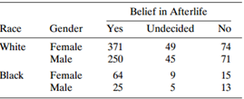
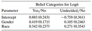
For Table 7.13, let Y = belief in life after death, x1= gender (1 = females, 0 = males), and x2= race (1 = whites, 0 = blacks). Table 7.14 shows the fit of the model log(πj/π3) = αj+ βjGx1+ βjRx2, j = 1, 2,with SE values in
A model fit predicting preference for U.S. President (Democrat, Republican, Independent) using x = annual income (in $10,000) is log(π̂D/π̂1) = 3.3 – 0.2x and log(π̂R/π̂1) = 1.0 + 0.3x.a. Find the prediction equation for log(π̂R/π̂D) and interpret the slope. For what range of x is
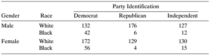
Table 7.15 refers to the effect on political party identification of gender and race. Find a baseline-category logit model that fits well. Interpret estimated effects on the odds that party identification is Democrat instead of Republican.Table 7.15: Party Identification Republican Gender Democrat
For 63 alligators caught in Lake George, Florida, Table 7.16 classifies primary food choice as (fish, invertebrate, other) and shows length in meters. Alligators are called subadults if length < 1.83 meters (6 feet) and adults if length > 1.83 meters.a. Measuring length as (adult, subadult),
For recent data from a General Social Survey, the cumulative logit model (7.5) with Y = political ideology (very liberal, slightly liberal, moderate, slightly conservative, very conservative) and x = 1 for the 428 Democrats and x = 0 for the 407 Republicans has β̂ = 0.975 (SE = 0.129) and α̂1 =
Refer to Problem 7.5. With adjacent-categories logits, β̂ = 0.435. Interpret using odds ratios for adjacent categories and for the (very liberal, very conservative) pair of categories.Data from Prob. 7.5:For recent data from a General Social Survey, the cumulative logit model (7.5) with Y =
Table 7.17 is an expanded version of a data set analyzed in Section 8.4.2. The response categories are (1) not injured, (2) injured but not transported by emergency medical services, (3) injured and transported by emergency medical services but not hospitalized, (4) injured and hospitalized but did
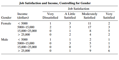
Refer to the cumulative logit model for Table 7.8.a. Compare the estimated income effect β̂1 = €“0.510 to the estimate after collapsing the response to three categories by combining categories (i) very satisfied and moderately satisfied, and (ii) very dissatisfied
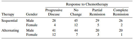
Table 7.19 refers to a clinical trial for the treatment of small-cell lung cancer. Patients were randomly assigned to two treatment groups. The sequential therapy administered the same combination of chernotherapeutic agents in each treatment cycle; the alternating therapy had three different
Table 9.7 displays associations among smoking status (S), breathing test results (B), and age (A) for workers in certain industrial plants. Treat B as a response.a. Specify a baseline-category logit model with additive factor effects of S and A. This model has deviance G2 = 25.9. Show that df = 4,
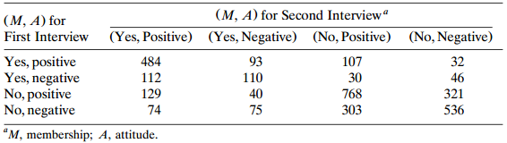
The book’s Web site (www.stat.ufl.edu/ ∼aa/cda/cda.html) has a 7 × 2 table that refers to subjects who graduated from high school in 1965. They were classified as protestors if they took part in at least one demonstration, protest march, or sit-in, and classified according to their party
For Table 7.5, the cumulative probit model has fit Φ€“1[PÌ‚(Y ‰¤ j)] = α̂j€“ 0.195x1+ 0.683x2, with α̂1= €“0.161, α̂2= 0.746, and
Table 7.21 shows results of fitting the mean response model to Table 7.8 using scores (3, 10, 20, 35} for income and (1, 3, 4, 5) for job satisfaction. Interpret the income effect, provide a confidence interval for the difference in mean satisfaction at income levels 35 and 3, controlling for
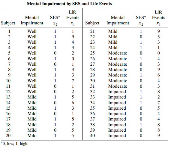
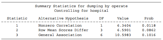
The book€™s Web site (wvvw.stat.ufl.edu/ ˆ¼aa/cda/cda.html) has a 3 × 4 × 4 table that cross-classifies dumping severity (Y) and operation (X) for four hospitals (H). The four operations refer to treatments for duodenal ulcer patients and have a
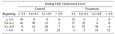
Table 7.23 refers to a study that randomly assigned subjects to a control or treatment group. Daily during the study, treatment subjects ate cereal containing psyllium. The study analyzed the effect on LDL cholesterol.a. Model the ending cholesterol level as a function of treatment, using the
A multivariate generalization of the exponential dispersion family (4.14) is f(yi; θi, ϕ) = exp{[yi’ θi – b(θi)]/α(ϕ) + c(yi, ϕ)}, where θi is the natural parameter. Show that the multinomial variate yi defined in Section 7.1.5 for a single trial with parameters {πj, j = 1,..., j –
Is the proportional odds model a special case of a baseline-category logit model? Explain why or why not.
Prove factorization (7.15) for the multinomial distribution.
Show that for the model, logit[P(Y ≤ j)] = αj + βjx, cumulative probabilities may be misordered for some x values.
For an I × J contingency table with ordinal Y and scores {xi = i} for x, consider the model logit[P(Y ≤ j | X = xi)] = αj + βxi.a. Show that residual df = IJ – I – J.b. Show that independence of X and Y is the special case β = 0.
F1(y) = 1 – exp (– λy) for y > 0 is a negative exponential cdf with parameter λ, and F2(y) = 1 – exp(– µy) for y > 0. Show that the difference between the cdf’s on a complementary log-log scale is identical for all y. Give implications for categorical data analysis.
When X and Y are ordinal, explain how to test conditional independence by allowing a different trend in each partial table.
For an I × J table, let ηij = log µij, and let a dot subscript denote the mean for that index (e.g., ηi. = ∑j ηij/J). Then, let λ = η.., λiX = ηi.– η.., λjY = η.j – η.., and λijXY = ηij – ηi. – η.j + η..·a. For 2 × 2 tables, show that log θ = 4λ11XY.b. For 2 ×
Suppose that all µijk> 0. Let ηijk= log µijk, and consider model parameters with zero-sum constraints.a. For model (XY, XZ, YZ) with a 2 × 2 × 2 table, show that λ11XY = 1/4 log θ11(k).b. For (XYZ) with a 2
Two balanced coins are flipped, independently. Let X = whether the first flip resulted in a head (yes, no), Y = whether the second flip resulted in a head, and Z = whether both flips had the same result. Using this example, show that marginal independence for each pair of three variables does not
For three categorical variables X, Y, and Z:a. Prove that mutual independence of X, Y, and Z implies that X and Y are both marginally and conditionally independent.b. When X is independent of Y and Y is independent of Z, does it follow that X is independent of Z? Explain.c. When any pair of
A 2 × 2 × 2 table satisfies πi++ = π+j+ = π++k = ½, all i, j, k. Give an example of {πijk} that satisfies model (a) (X, Y, Z), (b) (XY, Z), (c) (XY, YZ), (d) (XY, XZ, YZ), (e) (XYZ), but in each case not a simpler model.
Show that the general loglinear model in T dimensions has 2T terms. [It has an intercept, (T1) single-factor terms, (T2) two-factor terms,....]
Each of T responses is binary. For dummy variables {z1,..., zT}, the loglinear model of mutual independence has the form log µz1,....,zT = λ1 z1 + ... λT zT. Show how to express the general loglinear model.
Consider a cross-classification of W, X, Y, Z.a. Explain why (WXZ, WYZ) is the most general loglinear model for which X and Y are conditionally independent.b. State the model symbol for which X and Y are conditionally independent and there is no there-factor interaction.
For a four-way table with binary response Y, give the equivalent loglinear and logit models that have:a. Main effects of A, B, and C on Y.b. Interaction between A and B in their effects on Y, and C has main effects.c. Repeat part (a) for a nominal response Y with a baseline-category logit model.
For a 3 × 3 table with ordered rows having scores {xi}, identify all terms in the generalized loglinear model (8.18) for models (a) logit[P(Y ≤ j)] = αj + βxi, and (b) log [P(Y = j)/P(Y = 3)] αj + βj xi.
For the independence model for a two-way table, derive minimal sufficient statistics, likelihood equations, fitted values, and residual df.
For model (XV, Z), derive (a) minimal sufficient statistics, (b) likely hood equations, (c) fitted values, and (d) residual df for tests of fit.
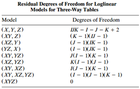
Verify the df values shown in Table 8.14 for models (XY, Z), (XY, YZ), and (XY, XZ, YZ).Table 8.14: Residual Degrees of Freedom for Loglinear Models for Three-Way Tables Model Degrees of Freedom (Х, У, Z) (XY, Z) (XZ, Y) (YZ, X) (XY, YZ) (XZ, YZ) (XY, XZ) (XY, XZ, YZ) (XYZ) IJK -1-J- K + 2 (к -
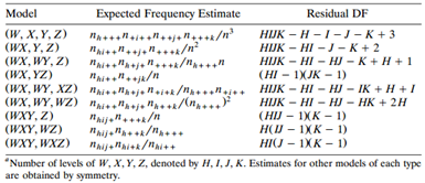
Table 8.22 shows fitted values for models for four-way tables that have direct estimates.a. Use Birch€™s results to verify that the entry is correct for (W, X, Y, Z). Verify its residual df.b. Motivate the estimate and df formulas for (WX, YZ), (WXY, Z), (WXY, WZ), and (WXY, WXZ) using
A T-dimensional table (nab...t) has Ii categories in dimension i.a. Find minimal sufficient statistics, ML estimates of cell probabilities, and residual df for the mutual independence model.b. Find the minimal sufficient statistics and residual df for the hierarchical model having all two-factor
Apply IPF to model (a) (X, YZ), and (b) (XZ, YZ). Show that the ML estimates result within one cycle.
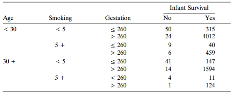
Table 9.17 summarizes a study with variables age of mother (A), length of gestation (G) in days, infant survival (I), and number of cigarettes smoked per day during the prenatal period (S). Treat G and I as response variables and A and S as explanatory.a. Explain why a loglinear model should
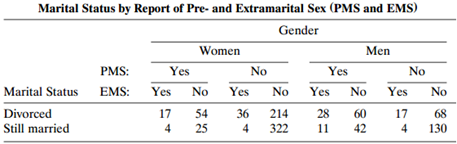
Consider the loglinear model selection for Table 6.3.a. Why is it not sensible to consider models omitting the λGM term?Table 6.3: Marital Status by Report of Pre- and Extramarital Sex (PMS and EMS) Gender Women Yes Men PMS: EMS: No Yes No Yes Marital Status Divorced Still married
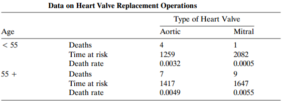
For Table 9.11, fit a model in which death rate depends only on age. Interpret the age effect.Table 9.11: Data on Heart Valve Replacement Operations Type of Heart Valve Aortic 4 1259 Mitral Age Deaths Time at risk Death rate Deaths Time at risk Death rate < 55 2082 0.0032 0.0005 55 + 1417 1647
Consider model (9.18). What is the effect on the model parameter estimates, their standard errors, and the goodness-of-fit statistics when (a) The times at risk are doubled, but the numbers of deaths stay the same; (b) The times at risk stay the same, but the numbers of deaths double; and (c) The
Showing 200 - 300
of 540
1
2
3
4
5
6
Step by Step Answers