New Semester
Started
Get
50% OFF
Study Help!
--h --m --s
Claim Now
Question Answers
Textbooks
Find textbooks, questions and answers
Oops, something went wrong!
Change your search query and then try again
S
Books
FREE
Study Help
Expert Questions
Accounting
General Management
Mathematics
Finance
Organizational Behaviour
Law
Physics
Operating System
Management Leadership
Sociology
Programming
Marketing
Database
Computer Network
Economics
Textbooks Solutions
Accounting
Managerial Accounting
Management Leadership
Cost Accounting
Statistics
Business Law
Corporate Finance
Finance
Economics
Auditing
Tutors
Online Tutors
Find a Tutor
Hire a Tutor
Become a Tutor
AI Tutor
AI Study Planner
NEW
Sell Books
Search
Search
Sign In
Register
study help
mathematics
categorical data analysis
Categorical Data Analysis 2nd Edition Alan Agresti - Solutions
Suppose that P(T = tj) = πj, j = 1 Show that E(mid-P-value) 0.5. [Show that ∑jπj(πj/2 + πj+1 + .....) = (∑jπj)2/2.]
Show that the moment generating function (mgf) for the binomial distribution is m(t) = (1 – π + πet)n, and use it to obtain the first two moments. Show that the mgf for the Poisson distribution is m(t) = exp{µ[exp(t) – 1]}, and use it to obtain the first two moments.
For the multinomial distribution, show thatShow that corr(n1, n2) = €“1 when c = 2. corr (n , n)- -η π.//π1-)Τ1- π).
Suppose that P(Yi = 1) = 1 – P(Yi = 0) = π, i = 1, . . . , n, where {Yi} are independent. Let Y = ∑i Yi).a. What are var(Y) and the distribution of Y?b. When {Yi} instead have pairwise correlation ρ > 0, show that var(Y) > nπ(1 – π), overdispersion relative to the binomial.
Why is it easier to get a precise estimate of the binomial parameter π when it is near 0 or 1 than when it is near 1/2?
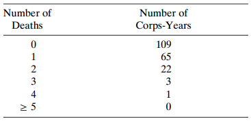
Table 1.3 contains Ladislaus von Bortkiewicz€™s data on deaths of soldiers in the Prussian army from kicks by army mules (Fisher 1934; Quine and Seneta 1987). The data refer to 10 army corps, each observed for 20 years. In 109 corps-years of exposure, there were no deaths, in 65
In a crossover trial comparing a new drug to a standard, π denotes the probability that the new one is judged better. It is desired to estimate π and test H0: π = 0.5 against Ha: π ≠ 0.5. In 20 independent observations, the new drug is better each time.a. Find and sketch the likelihood
Refer to the vegetarianism example in Section 1.4.3. For testing H0: π = 0.5 against H0: π ≠ 0.5, show that:a. The likelihood-ratio statistic equals 2[25log(25/12.5)] = 34.7.b. The chi-squared form of the score statistic equals 25.0.c. The Wald z or chi-squared statistic is infinite.
Consider the statement, “Please tell me whether or not you think it should be possible for a pregnant woman to obtain a legal abortion if she is married and does not want any more children.” For the 1996 General Social Survey, conducted by the National Opinion Research Center (NORC), 842
In his autobiography A Sort of Life, British author Graham Greene described a period of severe mental depression during which he played Russian Roulette. This “game’s consists of putting a bullet in one of the six chambers of a pistol, spinning the chambers to select one at random, and then
An experiment studies the number of insects that survive a certain dose of an insecticide, using several batches of insects of size n each. The insects are sensitive to factors that vary among batches during the experiment but were not measured, such as temperature level. Explain why the
Each of 100 multiple-choice questions on an exam has four possible answers, one of which is correct. For each question, a student guesses by selecting an answer randomly.a. Specify the distribution of the student’s number of correct answers.b. Find the mean and standard deviation of that
Identify each variable as nominal, ordinal, or interval.a. UK political party preference (Labour, Conservative, Social Democrat)b. Anxiety rating (none, mild, moderate, severe, very severe)c. Patient survival (in number of months)d. Clinic location (London, Boston, Madison, Rochester, Montreal)e.
Show the normal distribution N(µ, σ2) with fixed σ satisfies family (4.1), and identify the components. Formulate the ordinary regression model as a GLM.
For binary observations, consider the model π(x) = 1/2 + (1/π)tan–1(α + βx). Which distribution has cdf of this form? Explain when a GLM using this curve might be more appropriate than logistic regression.
Consider the value β̂ that maximizes a function L( β). Let β0 denote an initial guess.a. Using L’( β̂.) = L’( β(0) + (β̂ – β(0) L”(β(0)) + ..., argue that for β(0) close to β̂, approximately 0 = L’( β(0)) + (β̂ – β(0)) L’’(β(0)).Solve this equation to obtain
For n independent observations from a Poisson distribution, show that Fisher scoring gives µ(t + 1) = y̅ for all t > 0. By contrast, what happens with Newton—Raphson?
In a GLM, suppose that var(Y) = υ(µ) for µ = E(Y). Show that the link g satisfying g’(µ.) = [υ(µ)]–1/2 has the same weight matrix W(t) at each cycle. Show this link for a Poisson random component is g(µ) = 2√µ.
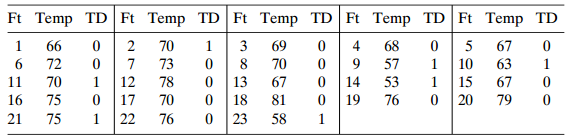
For the 23 space shuttle flights before the challenger mission disaster in 1986, Table 5.12 shows the temperature at the time of the flight and whether at least one primary O-ring suffered thermal distress.a. Use logistic regression to model the effect of temperature on the probability of thermal
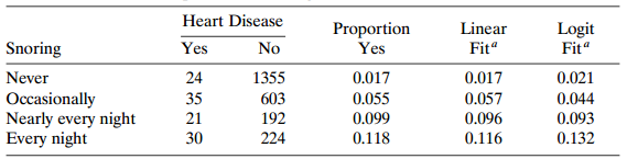
Refer to Table 4.2. Using scores {0, 2, 4, 5) for snoring, fit the logistic regression model. Interpret using fitted probabilities, linear approximations, and effects on the odds. Analyze the goodness of fit.Table 4.2:
Hastie and Tibshirani described a study to determine risk factors for kyphosis, severe forward flexion of the spine following corrective spinal surgery. The age in months at the time of the operation for the 18 subjects for whom kyphosis was present were 12, 15, 42, 52, 59, 73, 82, 91, 96, 105,
Refer to Table 6.11. The Pearson test of independence has X2(I) = 6.88. For equally spaced scores, the Cochran€”Armitage trend test has z2= 6.67 (P = 0.01). Interpret, and explain why results differ so. Analyze the data using a linear logit model. Test independence using the Wald and
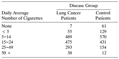
Refer to Table 2.11. Using scores (0, 3, 9.5, 19.5, 37, 55) for cigarette smoking, analyze these data using a logit model. Is the intercept estimate meaningful? Explain.Table 2.11: Disease Group Lung Cancer Patients Daily Average Number of Cigarettes Control Patients None 61 < 5 55 129 5-14 489 570
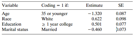
A study used the 1998 Behavioral Risk Factors Social Survey to consider factors associated with women€™s use of oral contraceptives in the United States. Table 5.13 summarizes effects for a logistic regression model for the probability of using oral contraceptives. Each predictor uses a
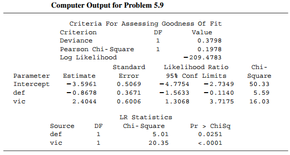
Refer to Table 2.6. Table 5.14 shows the results of fitting a logit model, treating death penalty as the response (1 = yes) and defendant€™s race (1 = white) and victims€™ race (1 = white) as dummy predictors.a. Interpret parameter estimates. Which group is most likely to have
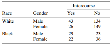
Table 5.15 appeared in a national study of 15-and 16-year-old adoles cent. The event of interest is ever having sexual intercourse, Analyze, including description and inference about the effects of gender and race, goodness of fit, and summary interpretations.Table 5.15: Intercourse Race Gender Yes
The National Collegiate Athletic Association studied graduation rates for freshman student athletes during the 1984–1985 academic year. The (sample size, number graduated) totals were (796, 498) for white females, (1625, 878) for white males, (143, 54) for black females, and (60, 197) for black
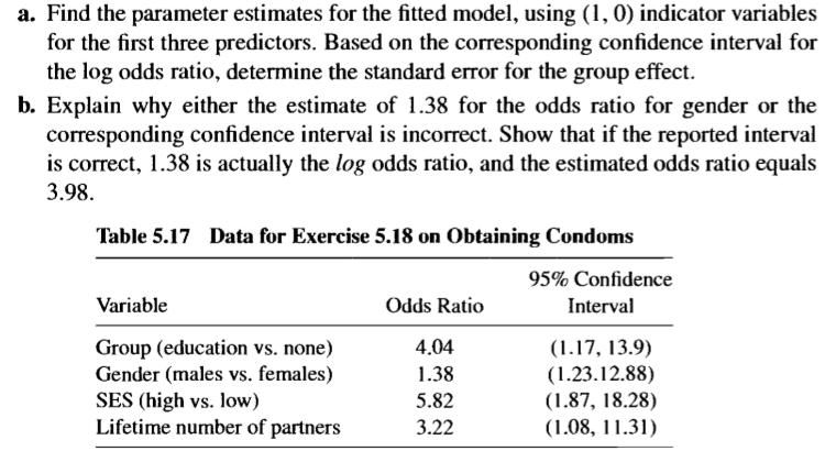
Ina study designed to evaluate whether an educational program makes sexually active adolescents more likely to obtain condoms, adolescents were randomly assigned to two experimental groups. The educational program, involving a lecture and videotape about transmission of HIV, was provided to one
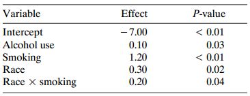
Table 5.17 shows estimated effects for a logistic regression model with squamous cell esophageal cancer (Y = 1, yes; Y = 0, no) as the response. Smoking status (S) equals 1 for at least one pack per day and 0 otherwise, alcohol consumption (A) equals the average number of alcoholic drinks consumed
A survey of high school students on Y = whether the subject has driven a motor vehicle after consuming a substantial amount of alcohol (1 = yes), s = gender (1 = female), r = race (1 = black: 0 = white), and g = grade (g1 = 1, grade 9; g2 = 1, grade 10; g3 = 1, grade 11; g1 = g2 = g3 = 0, grade 12)
Refer to model (5.2) for the horseshoe crabs using x = width.a. Show that (I) at the mean width (26.3), the estimated odds of a satellite equal 2.07; (ii) at x = 27.3, the estimated odds equal 3.40; and (iii) since exp(β̂ ) = 1.64, 3.40 = (1.64)2.07, and the odds increase by 64%.b. Based on the
Refer to the prediction equation logit(π̂) = – 10.071 – 0.509c + 0.458x for model (5.13). The means and standard deviations are c̅ = 2.44 and s = 0.80 for color, and x̅ = 26.30 and s = 2.11 for width.For standardized predictors [e.g., x = (width – 26.3)/2.11], explain why the estimated
Let Y denote a subject’s opinion about current laws legalizing abortion (1 = support), for gender h (h = 1, female; h = 2, male), religious affiliation i (i = 1, Protestant: i = 2, Catholic; i = 3, Jewish), and political party affiliation j (j = 1, Democrat; j = 2, Republican; j = 3,
For model (5.1), show that ∂π(x)/∂x = βπ(x)[1 – π(x)].
For model (5.1), when π(x) is small, explain why you can interpret exp(β) approximately as π(x + 1)/π(x).
Prove that the logistic regression curve (5.1) has the steepest slope where π(x) = 1/2. Generalize to model (5.8).
The calibration problem is that of estimating x at which π(x) = π0. For the linear logit model, argue that a confidence interval is the set of x values for which |α̂ + β̂x – logit(π0)|/[var(α̂) + x2 var(β̂) + 2x cov(α̂, β̂)]1/2 < zα/2.
A study for several professional sports of the effect of a player’s draft position d (d = 1, 2, 3,...) of selection from the pool of potential players in a given year on the probability π of eventually being named an all star used the model logit(π) = a + β log d.a. Show that π/(1 – π) =
Construct the log-likelihood function for the model logit[π(x)] = α + βx with independent binomial outcomes of y0 successes in n1 trials at x = 0 and y1 successes in n1 trials at x = 1. Derive the likelihood equations, and show that β̂ is the sample log odds ratio.
Suppose that Y has a bin(n,π ) distribution. For the model, logit(π) = α, consider testing H0: α = 0 (i.e., π = 0.5). Let π̂ = y/n.a. From Section 3.1.6, the asymptotic variance of α̂ = logit(π̂) is [nπ(l – π)]–1. Compare the estimated SE for the Wald test and the SE using the null
Showing 500 - 600
of 540
1
2
3
4
5
6
Step by Step Answers