New Semester
Started
Get
50% OFF
Study Help!
--h --m --s
Claim Now
Question Answers
Textbooks
Find textbooks, questions and answers
Oops, something went wrong!
Change your search query and then try again
S
Books
FREE
Study Help
Expert Questions
Accounting
General Management
Mathematics
Finance
Organizational Behaviour
Law
Physics
Operating System
Management Leadership
Sociology
Programming
Marketing
Database
Computer Network
Economics
Textbooks Solutions
Accounting
Managerial Accounting
Management Leadership
Cost Accounting
Statistics
Business Law
Corporate Finance
Finance
Economics
Auditing
Tutors
Online Tutors
Find a Tutor
Hire a Tutor
Become a Tutor
AI Tutor
AI Study Planner
NEW
Sell Books
Search
Search
Sign In
Register
study help
business
a course in statistics with r
A Course In Statistics With R 1st Edition Prabhanjan N. Tattar, Suresh Ramaiah, B. G. Manjunath - Solutions
For the galton dataset from UsingR package, what will be the conclusion of the MP test that the height of the child is H ∶ χ = 68 against K ∶ χ = 75, given that variance is known to be 1.7873.
If the variance is unknown in the previous example, carry out the likelihood-ratio test, see LRNormalMean_UV, and draw the conclusion at the χ = 0.05 level of significance.
Compare the Behrens-Fisher test results with the Mann-Whitney nonparametric test for the Youden-Beale data.
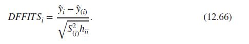
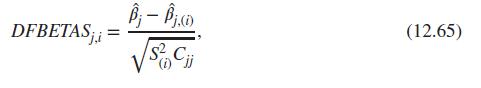
Using self-defined functions for DFFITS and DFBETAS, as given in Equations 12.66 and 12.65, say my_dffits and my_dfbetas, compute the values for an ailm fitted object and compare the results with the R functions dffits and dfbetas.Data from in Equation 12.66Data from in Equation 12.65
The VIF given in Equation 12.67 for a covariate requires computation of R2, as obtained in the regression model when the covariate is an output and other covariates are input variables for it. Thus, using 1/(1-summary (lm(xi∼x1+...+xi-1+xi+1+...+xp)) $r. squared), the VIF of the covariate xi may
Identify if the multicollinearity problems exist for the fitted ailm object using (i) VIF method, and (ii) eigen system analysis.
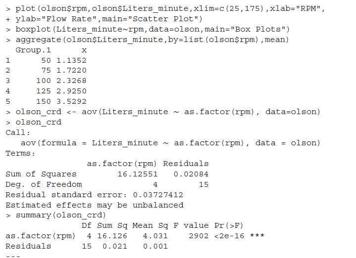
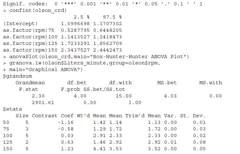
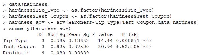
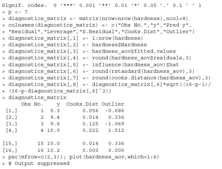
Carry out the diagnostic tests for the olson_crd fitted model in Example 13.3.4. Repeat a similar exercise for the ANOVA model fitted in Example 13.3.2.Data from in Example 13.3.4We need to determine the effect of the number of revolutions per minute (rpm) of the rotary pump head of an Olson
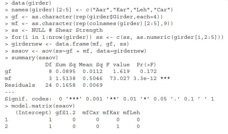
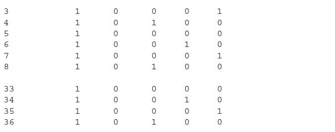
The function granova.2w may be applied on the girdernew dataset with a slight modification. Create a new data frame girdernew2 <- girdernew[,c(3,1,2)]. Note that an additional R package rgl will be required though. Test the code granova.2w( girdernew2, ss gf + mf) and make an attempt to
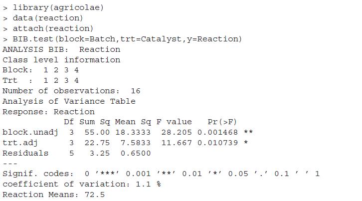
Perform the diagnostic tests on the BIBD model in Example 13.4.4.In Example 13.4.4For a chemical reaction experiment, the blocks arise due to the Batch number, Catalyst of different types from the treatments, and the reaction time is the output. Due to a restriction, all the catalysts cannot be
The Mahalanobis distance D2 given in Equation 14.7 is easily obtained in R using the mahalanobis function. Using this function, obtain the distance of the observations from the entire dataset for the board stiffness dataset and investigate for presence of outliers. Repeat the exercise for the
Using the HotellingsT2 function from the ICSNP package, test whether average sepal and petal length and width for setosa species equals [5.936 2.770 4.260 1.326] in the iris dataset.
Using the HotellingsT2 function from the ICSNP package, test whether average sepal and petal length and width for setosa species equals that of versicolor in the iris dataset.
Test whether the Sepal and Petal characteristics are independent of each other in the iris dataset.
Find the PCs for the stack loss dataset, which explain 85% of the variation in the original dataset.
For the US crime data of Example 13.4.2, carry out the PCA for the covariates and then perform the regression analysis on the PC scores. Investigate if the multicollinearity problem persists in the fitted regression model based on the PC scores.Data from in Example 13.4.2Consider the girder
Check out for the example of the factanal function. Are factors present in the iris dataset? Develop the complete analysis for the problem.
Perform the χ2 tests for the datasets in the first problem here.
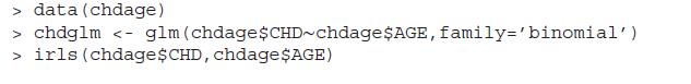
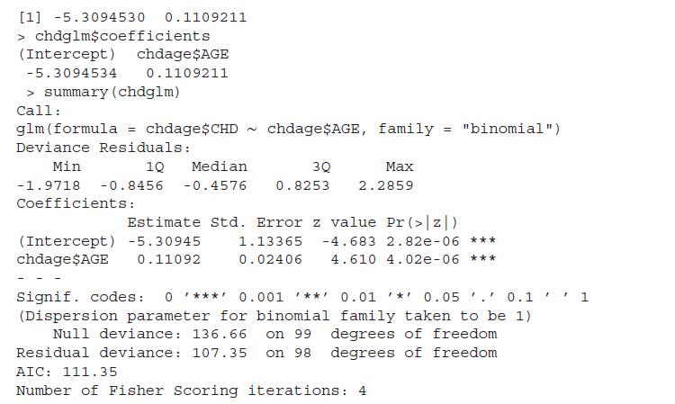
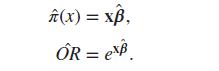
Obtain the 90% confidence intervals for the logistic regression model chdglm, as discussed in Example 17.5.1. Also, carry out the deviance test to find if the overall fitted model chdglm is a significant model? Validate the assumptions of the logistic regression model.Data from in Example
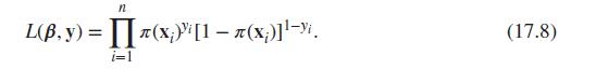
The likelihood function for the logistic regression model is given in Equation 17.8. It may be tempting to write a function, say lik_Logistic, which is proportional to the likelihood function. However, optimize does not return the MLE! Write a program and check if you can obtain the MLE.Data from
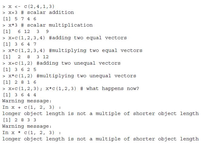
Write a program to obtain the minimum between two corresponding elements of two vectors. As an example, for the two vectors A=(1,2,3,4) and B=(4,3,2,1), your program should return the minimum as (1,2,2,1). Repeat the exercise to obtain the maximum. After you are done with your program, use the pmin
Using the options, fix the number of digits of the output during a session to four digits.
Find the details about complex numbers and perform the basic arithmetic related to complex numbers. What do you expect when you perform mean, median, and sd on an array of complex numbers? Check the results in R console.
For a gamma integral, it is well known that Γ(n) = (n − 1)!, where n is an integer. Verify the same for your choice of integers. Note that you are required to use gamma for the left-hand side and the factorial function for the right-hand side.
For a number x, can you always say that round(floor(x)) == floor (ro und(x)). Also, test which of these relationships hold true: floor (ceil ing(x)) == ceiling(floor(x)), floor(sign(x)) == sign(floor(x)).
By using the is.na function to substitute the missing observations of a vector, you may select a numeric vector of your choice with missing values, with 0. Attempt to replace the missing values of a vector with the mean of the vector having valid elements.
Consider the factor vector explevels <- gl(3, 2), and now change the third and fourth elements to 1 with explevels[3:4]<-1. Now, 2 is an extra factor level which is not present as a factor for any of its elements. Drop it! Use droplevels.
For a numeric vector, do you expect min(x) == -max (-x) ?
The Stirling function stirling is given as an approximation of n!. The R function factorial is also an approximation for the factorial operation. This means that prod(1:n) will not always be the same as Πn j=1 j. Find out the least n for which factorial does not agree with the result for
In Subsection 2.4.1, we computed the norm of a vector x as sqrt (sum(x ̂ 2)). With some extra effort, it is indeed possible to obtain the same using the R function norm. Explore the options type and complete the use of the norm function which gives the same answer as sqrt(sum(x ̂ 2)).Data from in
Create the matrix A <- matrix(1:16,nrow=4) in R. Using the functions upper. tri, lower. tri, and diag, obtain the identity matrix.
For the matrix A<- matrix(c(1:12),nrow=2), find the determinant using the det function.
Check whether ginv and solve result in the same inverse matrix for a non-singular square matrix? In the case of a singular matrix, say matrix(rep(1,4),nrow=2), what will be the generalized inverse?
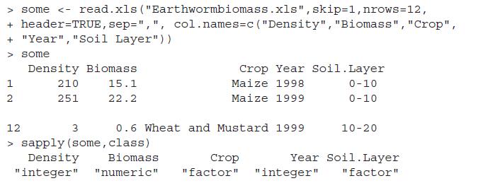
For the data. frame some in Example 3.2.2, what will be your expectation of the R code summary(some)? Validate the expectation by running the code too.Data from in Example 3.2.2In this example, we have a few more added complexities. Here, we have to skip the first line of the xls file, which is a
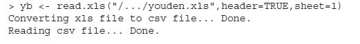
By considering the dataset rootstock imported in Section 3.3, export the data back to the working directory using the write. dta function from the foreign package.Data from in Section 3.3Datasets may be available in formats other than csv or dat. It is also a frequent situation where we need to
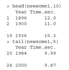
Run edit(newsome1) as required in Section 3.4, and comment on how this function is different from the View function.Data from in Section 3.4R objects are of varying nature and we may be interested in having a quick look at the dataset itself, and not through sophisticated tools such as graphics or
For any directory in your computer, use the function list. files to obtain the contents, inclusive of files and maybe other directories. Recollect that the default list. files () function returns the contents in the working directory, and hence you need to experiment with a directory other than
The attach function, when applied on a data. frame object, loads the variables in the R session. How do you undo this operation? If the attach function is repeated more than once, what will be the result?
Suppose that the option header=FALSE is an error when an object is imported. Write appropriate codes which bring up the right variable names and deletes the wrong observations too. For example, suppose that the chest data is inappropriately imported with chest <-read. csv ("Chest_VH.
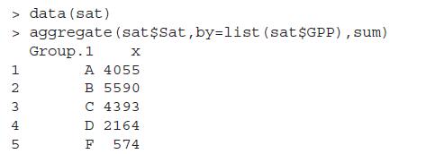
Using the aggregate function, as in Example 3.5.1, obtain the frequency instead of sum. Also, extend the list variables in the example to include both GPP and Grade, and hence obtain the sum of Sat for possible combinations of these two variables.Data from in Example 3.5.1We have the sat.csv fie
Using the ifelse conditional function, create a new as. Date type of function, which can read date objects available in a vector in two different forms.
Find the time difference between two time objects in units of hours, days, etc.
Let x be a numeric vector. Create a new function, say depth, which will have a serial number as an argument, between 1:length(x), and its output should return the depth of the datum.
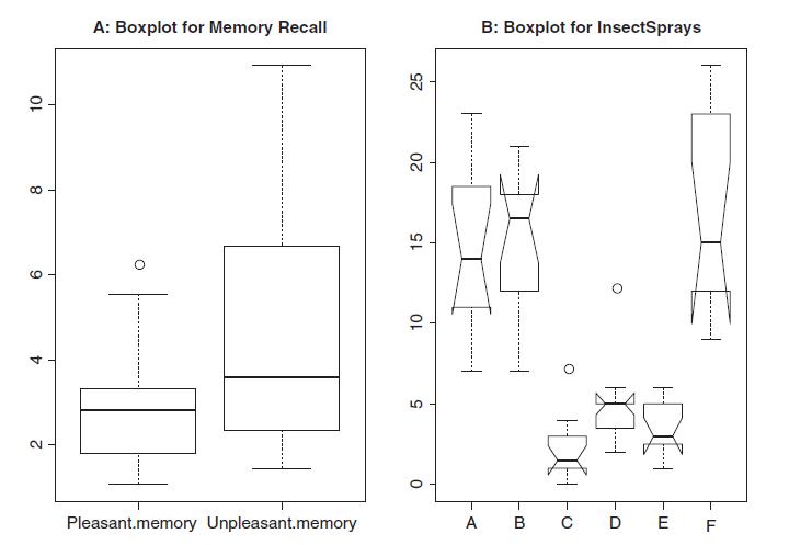
The part B of Figure 4.4, see Example 4.5, clearly shows the presence of outliers for the number of dead insects for insecticides C and D. Identify the outlying data points. Remove the outlying points, and then check if any more potential outliers are present.Data from in Figure 4.4Data from in
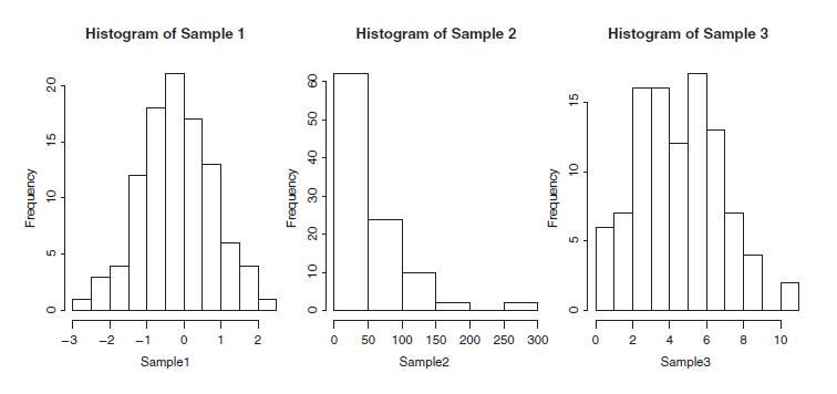
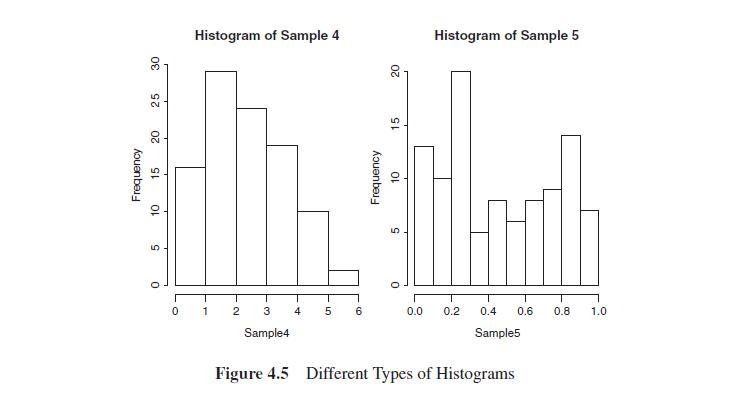
The number of intervals for the five histograms in Figure 4.5 can be seen as 11, 6, 11, 6, and 10. How do you obtain these numbers through R?Data from in Figure 4.5 5 5 0 -3 Histogram of Sample 1 T -2 T -1 T 0 Sample1 1 1 2 8 Ot 0 0 Histogram of Sample 2 50 100 150 200 250
Create a function which generates a histogram with the intervals according to the percentiles of the data vector.
Explore the different choices of breaks given in Formulas 4.5 – 4.7 for the different histogram examples.
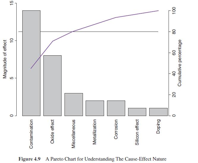
Using the R function pareto.chart from the qcc package, obtain the Pareto chart for the causes and frequencies, as in Example 4.10, and compare the results with Figure 4.9.Data from in Figure 4.9 Figure 4.9 A Pareto Chart for Understanding The Cause-Effect Nature Contamination Oxide
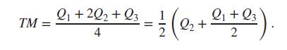
Create an R function, say trimean, for computing trimean, as given in Equation 4.8. Apply the new function for datasets of your choices considered in the chapter.Data from in Equation 4.8 TM Q₁ +222 +23 4 = 1/ (0₁₂+ ²₁ +0₁). 2
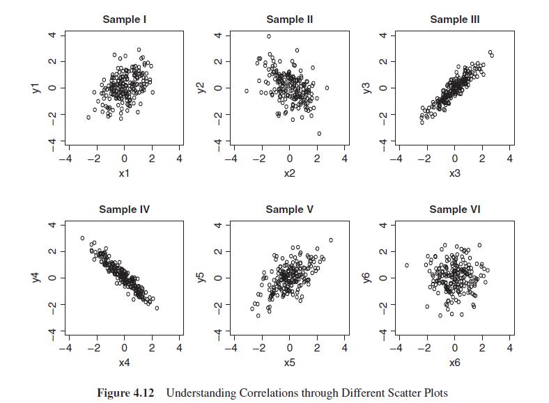
Fit resistant line models for the six pairs of data discussed in Example 4.17. Validate the correlations as implied by the scatter plots in Figure 4.12.Data from in Figure 4.12 LÁ y4 4 2 0 -2 -4 4 2 0 -2 -4 O 0 Sample I 000 -2 0 2 x1 -2 Sample
For the datasets available in the files rocket_propellant.csv and toluca_company.dat, build the resistant line models. In the former file, the input variable is Age_of_Propellant, while in the latter file it is Lot_Size. The output variables in these respective files are Shear_Strength and
Consider the three sets from Ω = LETTERS: A = {“U”, “X”, “M”, “J”, “B”, “D”}, B = {“N”, “J”, “H”, “C”, “G”, “X”}, and C = {“H”, “V”, “N”, “K”,“D”, “F”}. Using the operators intersect and union, for the sets A, B, and C, verify
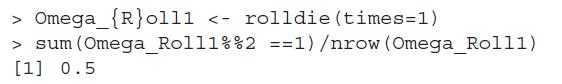
The sample space of a die rolling becomes very large, depending on number of times we roll the die, and also on the number of sides of the die. Write a R program using the rolldie function from the prob package, single line preferred, which returns the total number of possible outcomes for (i) a
Find out more details about the Roulette game and make a preliminary finding about it in the function roulette.
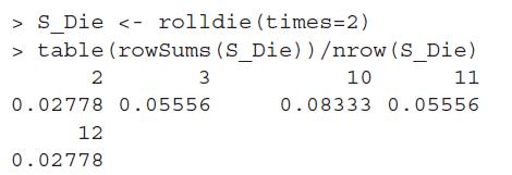
Run the codes names(table(rowSums(S_Die))) and table (rowSums(S_Die)) from Example 5.2.7 and verify that you have completely understood the examples code. Now, roll four die and answer the probability of obtaining an odd number greater than ten.Data from in Example 5.2.7Contd. For the rolling
For the thirteenth of a month problem, start with an arbitrary year, say 1857, and then run the program up to year 2256. Do you expect that the 13th will more likely be a Friday than any other day? Confirm your intuition with the R program.
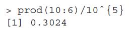
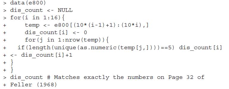
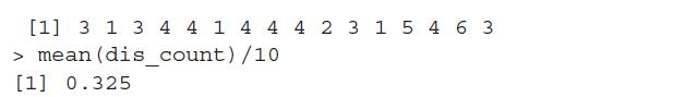
In Example 5.3.3, the digits are drawn to solve a replacement problem. Obtain the probability of obtaining at least two even numbers in a draw of five using the leading digits of e.Data from in Example 5.3.3Feller (1968), pages 31–2. Consider the population of 10 digits, 0, 1, … , 9. Suppose
What is the number of people whose birthday you need to ask so that the probability of finding a birthday mate is at least half? Write a brief R program to obtain the size as the probability varies from 0 to 1.
Construct a program which can conclude if the collection of sets over a finite probability space is a field.
Extend the program in the previous problem to verify if probabilities defined over an arbitrary collection of finite sets satisfies the requirement of being a probability measure.
Explore if the addrv function from the prob package can be used to handle more than two variables.
Extend the R function Expectation_NNRV_Unif for computing the expectation of a uniform RV over the interval [−a, a], a ∈ R.
Evaluate the R program of de Moivre-Laplace CLT for different values of p.
Using the normal approximation, CLT result, for the triangular distribution for various values of a, b, and c, create an R program for evaluating P(−c∕2 < X̄ < c∕2).
For the uniform and beta distribution, write R programs to obtain mean and variance using Equation 5.16.Data from in Equation 5.16 EX = EX+ - EX-,
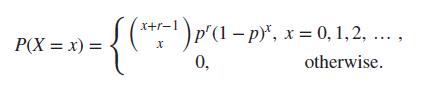
For a fixed p value in a negative binomial RV, see Equation 6.20, obtain a plot of the mean and variance for different r values and comment.Data from in Equation 6.20 (x+r-¹) p'(1 − p)*, x = 0, 1, 2, ..., { - 0, otherwise. P(X = x) =
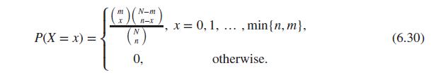
Using the choose function, create a new function for the pmf of hypergeometric distribution.
Using the integrate and dt (for density of t-distribution), verify the mean and variance of the t RV.
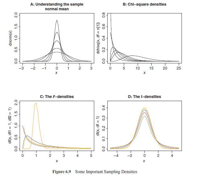
Reconstruct Part A of Figure 6.9 using the curve function instead of the plot function. What are the apparent advantages of using the curve function, if any?Data from in Figure 6.9 2.0 1.5 dnorm(x) 1.0 0.5 0.0 2.0 1.5 df(x, df1= 1, df2= 1) 1.0 0.5 0.0 -3 0 A: Understanding the sample normal
Suppose X follows a negative binomial distribution with parameters as defined in Equation 6.20. Assume that for obtaining r = 6 failures, x is noted as 10. Obtain the likelihood function plot and then graphically infer about the ML estimate of p.Data from in Equation 6.20 P(X= x) = x+r-1 +-¹) p'(1
In a directory on a particular folder of a hard disk drive, there are N = 50 files. Suppose that in a random selection of n = 12 files, 9 are observed to be e-books. Under the assumption of a hypergeometric distribution, and by using the likelihood function approach, give the ML estimate of m.
The t-test used on the galton dataset is t.test(galton$child,mu= mean(galton$parent)). However, there is a “pairing” between the height of the child and the parent. Is the test t.test(galton$child, galton$parent,paired=TRUE) more appropriate?
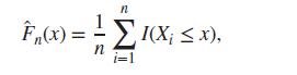
For the swiss $Bottforg data vector, obtain the empirical cdf and estimate the statistical functionals of skewness and kurtosis.
For the parent height in the galton set, obtain the histogram smoothing and the kernel smoothing estimates and draw the right inference.
The nerve dataset, as discussed in Section 8.2, deals with the cumulative distribution function. Estimate the density function of the nerve data using histogram smoothing, and uniform, Epanechnikov, biweight, and Gaussian kernels.Data from in Section 8.2Let X1, X2, … , Xn be a random sample
For a beta prior Be(a, b) on the probability of success in a Bernoulli trial, find the probability of sunrise. For a large n, obtain the plot of the probability for various a and b values.
Under a symmetric Dirichlet prior, with symmetric parameter c, the probability of a birthday match, see Diaconis and Holmes (2002) is given by Write an R program to compute the probability of a match when c is 0.5, 1, 2, 5, 20, 200. k-1 P¿(match) = 1 - ] (n − ¹)c nc + i i=1
The TPM of a gamblers walk consists of infinite states. Restricting the matrix over [−n, n] states, that is considering only the corresponding rows and columns and not the restricted gamblers walk, obtain the digraph using the sna package.
Using the msteptpm function, obtain P10 for testtpm, testtpm2, and testtpm3 TPM’s.
Using the p.as.plot function from Convergence Concepts, study the convergence in probability and almost sure convergence limit theorems.
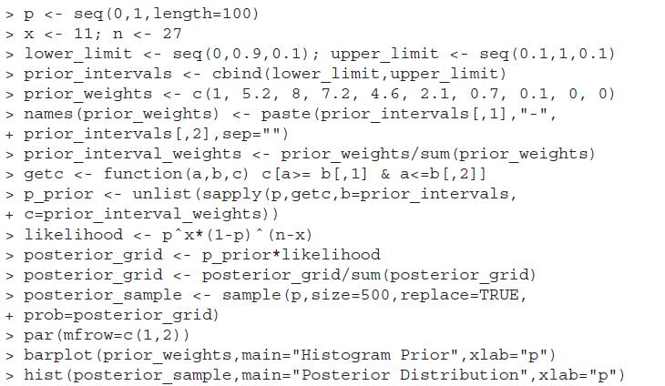
Elaborate on the details of the R program in Example 11.6.1.Data from in Example 11.6.1The prior probability prior_weights is extended over a prior grid as required in this approach. A very elementary function getc helps in this task along with the sapply function. The likelihood function is
Simulate 1000 observations from the standard normal distribution using AR_Normal function and then obtain the histogram with the option freq=FALSE (why?). Add the normal curve, try curve with add=TRUE option, and check if the simulated observations are satisfactory?
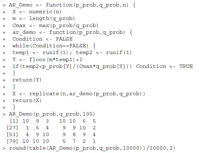
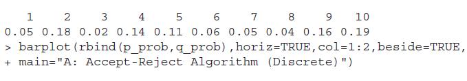
Using the accept-reject algorithm, generate observations from the binomial distribution as target distribution and the uniform distribution as proposal distribution. Reverse the roles and carry out the simulation and note the differences, if any.Data is accept-reject algorithmSimulation from
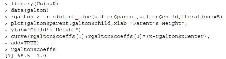
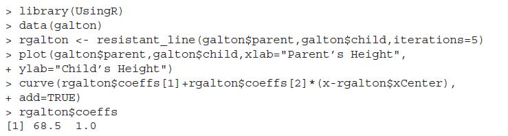
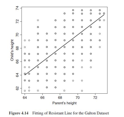
Fit a simple linear regression model for the Galton dataset as seen in Example 4.5.1. Compare the values of the regression coefficients of the linear regression model for this dataset with the previously obtained resistant line coefficients.Data from in Example 4.5.1This dataset was used earlier as
Extend the concept of R2 and AdjR2 for the resistant line model. Create an R function which will extract these two measures for a fitter resistant line model and obtain these values for the Galton dataset, rp, and tc.
The Sign if. codes as obtained by summary (lm) may be easily customized in R to use your own cut-off points, and symbols too. There are two elements to this, first the cut-off points for the p-values and the default settings are cutpoints = c(0, 0.001, 0.01, 0.05, 0.1, 1), and the second part has
In Example 13.4.3, change the range of the variables x1 and x2 to x1 <- rep(seq(-10,10,0.5),100) and x2 <- rep(seq(-10,10, 0.5),each=100) and redo the three-dimensional plot, especially for the third linear regression model. Similarly, for the contour plot of the same model, change the
For the fitted linear model crime_rate_lm, using the usc dataset, obtain the plot of residuals against the fitted values.
Verify the properties of the hat matrix H given in Equation 12.37 for the fitted object crime_rate_lm, or any other fitted multiple linear regression model of your choice.Data from in Equation 12.37 H = X(X'X)-¹X'. (12.37)
Identify which of the design models studied in this chapter are appropriate for the datasets available in the BHH2 package. The list of datasets available in the package may be found with try(data(package="BHH2")). The exercise may also be repeated for design-related packages such as agricolae,
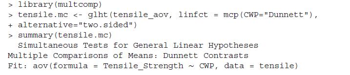
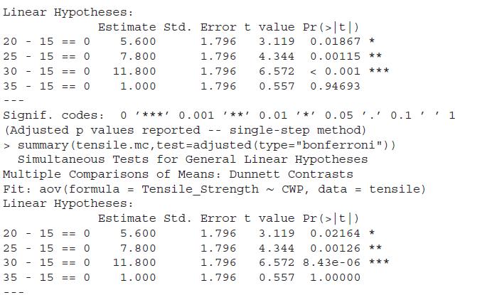
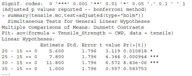
Multiple comparison tests of Dunnett, Tukey, Holm, and Bonferroni have been explored in Example 13.3.8. The confidence intervals are reported only for Tukey HSD. The reader should obtain the confidence intervals for the rest of the multiple comparison tests contrasts.Data from in Example
Explore the use of the functions design.crd and design.rcbd from the agricolae package for setting up CRD and block designs.
The iris data has been introduced in AD2. Obtain the matrix of scatter plots for (i) the overall dataset (removing the Species), and (ii) three subsets according to the Species. Obtain the average of the four characteristics by the Species group and using the faces function from the aplpack
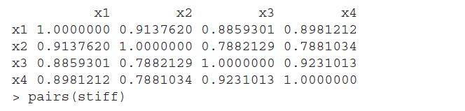
For the board stiffness data discussed in Example 14.3.3, obtain the covariance matrix and then using the cov2cor function, obtain the correlation matrix.Data from in Example 14.3.3Four measures of stiffness of 30 boards are available. The first measure of stiffness is obtained by sending a shock
Run the example code of the function HotellingsT2, that is run example(HotellingsT2), and explore the options available with this function.
Carry out the MANOVA analysis for the iris datasets, where the hypothesis problem is that the mean of the multivariate vector of the four variables are equal across the three types of species.
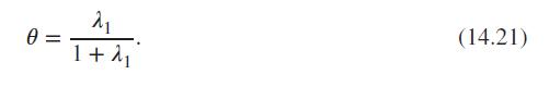
Using base matrix tools of R, create a function which returns the value of Roy’s test statistic given in Equation 14.21.Data from in Equation 14.21 e= 서 1+₁ (14.21)
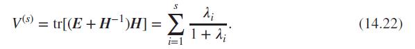
Repeat the above exercise for the Pillai and Lawley-Hotelling tests respectively given in Equations 14.22 and 14.23.Data from in Equations 14.22Data from in Equations 14.23 S λ; ΣΤΑ 1 + 2; i=l V(s) = tr[(E + H^^)H] = Σ (14.22)
Explore the R examples for linear discriminant analysis and canonical correlation with example (lda) and example (cancor).
Perform the PCA on the iris dataset along the two lines: (i) the entire dataset, (ii) three subsets according to the three species. Check whether the PC scores are significantly different across the three species using an appropriate multivariate testing problem.
Obtain stacked bar plots for UCB Admissions, Hair Eye Color, and Titanic datasets.
Showing 2200 - 2300
of 2302
First
10
11
12
13
14
15
16
17
18
19
20
21
22
23
24
Step by Step Answers