New Semester Started Get 50% OFF Study Help! --h --m --s Claim Now

Question Answers

Textbooks

Find textbooks, questions and answers

Oops, something went wrong!

Change your search query and then try again

Result Not Found

Books FREE
Study Help
Tutors
AI Study Planner NEW
Sell Books

Search
Sign In
Register

study help
engineering
introduction mechanical engineering

Mechanical Vibrations Theory And Applications 1st Edition S. GRAHAM KELLY - Solutions

What are the local generalized coordinates associated with a beam element.
How many degrees of freedom are there in a three-element model of a fixed-free bar?
How many degrees of freedom are there in a two-element model of a fixed-fixed shaft with a rotor at its midspan?
How many degrees of freedom are there in a two-element model of a fixed-fixed beam?
How many degrees of freedom are there in a two-element model of a fixedpinned beam?
How many degrees of freedom are there in a three-element model of a fixed-free beam?
How many degrees of freedom are there in a three-element model of beam fixed at one end and attached to a linear spring at its other end?
Use a one-element, finite-element model to approximate the lowest natural frequency of a bar (elastic modulus \(E\), density \(ho\), area \(A\) and length \(L\) ) that is fixed at one end and attached to a discrete spring of stiffness \(E A / 2 L\) at its other end.
Use a one-element, finite-element model to approximate the lowest torsional natural frequency of a uniform shaft with a length \(L\), polar moment of inertia \(J\), is made from an elastic material of density \(ho\), and has a shear modulus \(G\) that is fixed at one end and has a torsional spring
Use a one-element, finite-element model to approximate the lowest torsional natural frequency of a uniform shaft with a length \(L\) polar moment of inertia \(J\), is made from an elastic material of density \(ho\), and has a shear modulus \(G\) that is fixed at one end and has a rigid disk with a
Use a one-element, finite-element model to approximate the steady-state amplitude of a uniform bar with a length \(L\), cross-sectional area \(A\), is made from an elastic material of density \(ho\), and has an elastic modulus \(G\) that is fixed at one end and has harmonic force \(f(t)=F_{0} \sin
Develop the element mass matrix for a bar element that is circular in cross section but has a linearly varying radius over the element. The radius is \(r_{1}\) at \(\xi=0\) and is \(r_{2}\) at \(\xi=\ell\).
Develop the element stiffness matrix for a bar element that is circular in cross section but has a linearly varying radius over the element. The radius is \(r_{1}\) at \(\xi=0\) and is \(r_{2}\) at \(\xi=\ell\).
Develop the element mass matrix for a bar element that is made of a material of varying density. The density varies linearly over the element and is \(ho_{1}\) at \(\xi=0\) and \(ho_{2}\) at \(\xi=\ell\).
Use a one-element, finite-element model to predict the lowest natural frequency of a beam with a length \(L\), cross-sectional area \(A\), mass moment of inertia \(I\), is made from a material of mass density \(ho\), and has an elastic modulus \(E\) that is fixed at one end and attached to a linear
A concentrated load \(f(t)=F_{0} \sin \omega t\) is acting at the midspan of a simply supported beam with a length \(L\), cross-sectional area \(A\), mass moment of inertia \(I\), is made from a material of mass density \(ho\), and has an elastic modulus \(E\). Use a one-element, finite-element
A concentrated load \(f(t)=F_{0} \sin \omega t\) is applied to the end of a uniform fixedfree beam. Use a one-element, finite element model to predict the steady-state amplitude of displacement of the end of the beam.
The potential energy scalar product for a uniform bar is defined as\[(f, g)_{v}=\int_{0}^{L} E A f(x) \frac{d^{2} g}{d x^{2}} d x\]Consider the cases where(a) the bar is fixed at \(x=0\) and free at \(x=L\) and(b) the bar is fixed at \(x=0\) and attached to a linear spring of stiffness \(k\) at
Use the assumed modes method with trial functions\[ w_{1}(x)=\sin \left(\pi \frac{x}{L}\right) \quad w_{2}(x)=\sin \left(2 \pi \frac{x}{L}\right) \quad w_{3}(x)=\sin \left(3 \pi \frac{x}{L}\right) \]to approximate the lowest natural frequency and its corresponding mode shape for a uniform
Let \(w_{1}(x), w_{2}(x), w_{3}(x), w_{4}(x)\) be linearly independent polynomials of degree four or less that satisfy the geometric boundary conditions for a bar fixed at \(x=0\) and attached to a spring of stiffness \(k\) at \(x=L\).(a) Determine a set of \(w_{1}(x), w_{2}(x), w_{3}(x),
Use the assumed modes method with trial functions\[ w_{1}(x)=x(x-L) \quad w_{2}(x)=x(x-L)^{2} \quad w_{3}(x)=x(x-L)^{3} \]to approximate the two lowest natural frequencies and mode shapes for a simply supported beam.
Repeat Chapter Problem 11.4 if the beam has a machine of mass \(m=2.0 ho A L\) where \(ho A L\) is the total mass of the beam. The machine is placed at the midspan of the beam.Data From Chapter Problem 11.4:Use the assumed modes method with trial functions\[ w_{1}(x)=x(x-L) \quad
The mode shapes of a uniform fixed-free bar are of the form\[ \phi_{n}(x)=\sin \left[\frac{(2 n-1) \pi x}{2 L}\right] \quad n=1,2,3, \ldots \]Use the assumed modes method with \(\phi_{1}(x), \phi_{2}(x), \phi_{3}(x)\) as trial functions to approximate the lowest natural frequency and mode shapes
Use a one-element, finite-element model to approximate the lowest natural frequency of a uniform bar of mass density \(ho\), cross-sectional area \(A\), elastic modulus \(E\), and length \(L\) that is fixed at one end and has a block of mass \(m\) attached at one end.
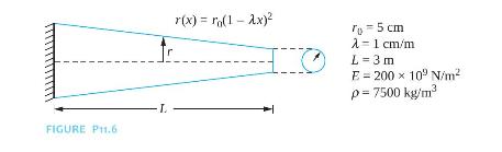
Derive the element stiffness and mass matrices for a tapered bar of rectangular cross-section, \(A(x)=A_{0}(1-\mu x)\).
Use a one-element, finite-element model to approximate the lowest nonzero torsional natural frequency of a uniform shaft of mass density \(ho\), polar moment of inertia \(J\), shear modulus \(G\), and length \(L\) that has a thin disk of mass moment of inertia \(I_{1}\) attached at one end and a
Use a one-element, finite-element model to approximate the lowest natural frequencies of a uniform beam of mass density \(ho\), cross-sectional area \(A\), crosssectional moment of inertia \(I\), elastic modulus \(E\), and length \(L\) that is free at both ends.
Derive the element \(m_{34}\) of the element mass matrix for a beam element.
Derive the element \(k_{23}\) of the element stiffness matrix for a beam element.
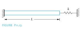
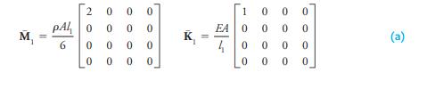
Use a two-element, finite-element model to approximate the two lowest natural frequencies and their corresponding mode shapes for the system of Figure P11.13.\[ \begin{aligned} & E=200 \times 10^{9} \mathrm{~N} / \mathrm{m}^{2} \\ & A=1.6 \times 10^{-4} \mathrm{~m}^{2} \\ & L=2.5
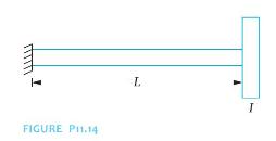
Use a two-element, finite-element model to approximate the two lowest torsional natural frequencies for the system of Figure P11.14.\[ \begin{aligned} & J=3.2 \times 10^{-5} \mathrm{~m}^{4} \\ & G=80 \times 10^{9} \mathrm{~N} / \mathrm{m}^{2} \\ & ho=7000 \mathrm{~kg} /
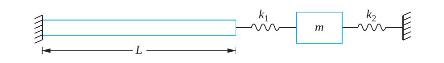
Use a three-element, finite-element model to approximate the lowest natural frequency and its corresponding mode shape for the system of Figure P11.15.\[ \begin{array}{ll} E=200 \times 10^{9} \mathrm{~N} / \mathrm{m}^{2} & m=1.2 \mathrm{~kg} \\ A=3.5 \times 10^{-5} \mathrm{~m}^{2} & k_{1}=2
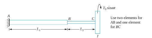
Use a three-element, finite-element model to approximate the steady-state response of the system of Figure P11.16.\[ \begin{array}{lll} L_{1}=2.1 \mathrm{~m} & L_{2}=1.0 \mathrm{~m} & I=0.25 \mathrm{~kg} \cdot \mathrm{m}^{2} \\ G_{1}=40 \times 10^{9} \mathrm{~N} / \mathrm{m}^{2} &
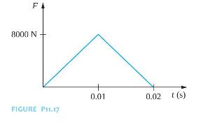
Use a three-element, finite-element model to approximate the forced response of the system of Figure P11.15 when the end of the bar is subject to the excitation of Figure P11.17.\[ \begin{array}{ll} E=200 \times 10^{9} \mathrm{~N} / \mathrm{m}^{2} & m=1.2 \mathrm{~kg} \\ A=3.5 \times 10^{-5}
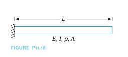
Use a two-element, finite-element model to approximate the two lowest natural frequencies of transverse vibration of the beam of Figure P11.18. -L FIGURE P11.18 E, I, p, A
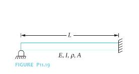
Use a two-element, finite-element model to approximate the lowest natural frequencies of the beam of Figure P11.19. L FIGURE P11.19 E, I. p. A
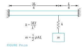
Use a two-element, finite-element model to approximate the two lowest natural frequencies of the system of Figure P11.20. Use elements of equal length. 3L 4 3E1 k m -PAL FIGURE P11.20 E
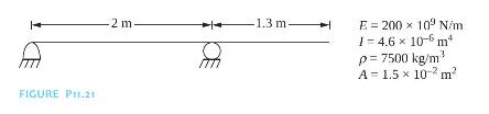
Use a three-element, finite-element model to approximate the three lowest natural frequencies of the system of Figure P11.21. FIGURE P11.21 2 m. 1.3 m E = 200 10 N/m 1-4.6 10-6 m p = 7500 kg/m A-1.5 10-2 m
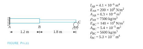
Use a two-element, finite-element model to approximate the lowest natural frequency of the system of Figure P11.22. A B 1.2 m 1 1.8 m T FIGURE P11.22 TAB=4.1 10m EAR 200 x 10 N/m AAB 6.3 10-4 m PAR = 7500 kg/m EBC 140 x 10 N/m ABC: 5.4 105 m PBC=5600 kg/m 4BC 5.3 x 107 m
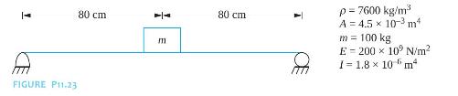
Use a two-element, finite-element model for the beam to approximate the two lowest natural frequencies of the system of Figure P11.23. T D FIGURE P11.23 80 cm E 80 cm T p = 7600 kg/m A 4.5 x 103 m4 m = 100 kg E 200 x 109 N/m 1= 1.8 105 m x
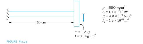
Use a two-element, finite-element model to approximate the two lowest natural frequencies of the system of Figure P11.24. FIGURE P11.24 60 cm T m = 1.2 kg I = 0.8 kg. m p = 8000 kg/m A 1.1 x 10m E-200 x 109 N/m Ib = 1.9 x 10 m
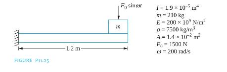
Use a three-element, finite-element model to approximate the steady-state amplitude of the machine of the system of Figure P11.25. FIGURE P11.25 1.2 m m Fo sincot 1=1.9 10m m = 210 kg E 200 x 10" N/m p = 7500 kg/m A=1.4 10- m F = 1500 N @ 200 rad/s
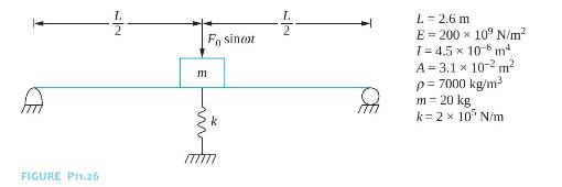
Use a three-element, finite-element model to approximate the steady-state amplitude of the machine of the system of Figure P11.26. L 2|2 Fo sincor FIGURE P11.26 m k 72 L = 2.6 m E 200x109 N/m T= 4.5 10-6 m4 A = 3.1 x 10-2 m p=7000 kg/m m = 20 kg k= 2 10 N/m
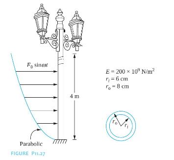
The street light has a mass of \(25 \mathrm{~kg}\). The wind velocity is \(60 \mathrm{~m} / \mathrm{s}\), but the force distribution is as shown in Figure P11.27. Use a three-element, finiteelement model of the structure to approximate the steady-state amplitude of the light. Fo sincor Parabolic
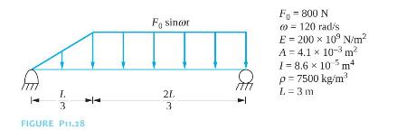
Use a three-element, finite-element model to approximate the steady-state response of the system of Figure P11.28. L - 3 FIGURE P11.28 11 F sincot 21. 23 F = 800 N = 120 rad/s E-200 x 109 N/m A = 4.1 10-3 m I 8.6 10 m p = 7500 kg/m L=3m
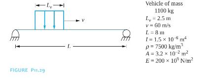
A plate and girder bridge is modeled as a simply supported beam, as illustrated in Figure P11.29. A vehicle is traveling across the bridge with the velocity \(v\). Use a three-element, finite-element model of the bridge to determine the time-dependent response of the structure as the vehicle is
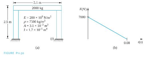
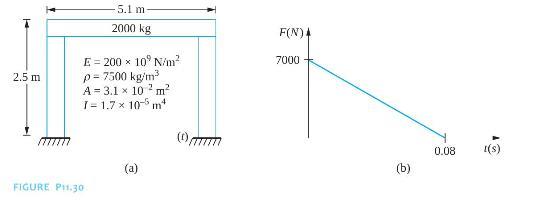
A simple model of a one-story frame structure is shown in Figure P11.30(a). Use one beam element to model each of the columns and two bar elements to model the girder. Determine the response of the structure if it is subject to the blast force of Figure P11.30(b). 2.5 m FIGURE P11.30 5.1 m 2000 kg
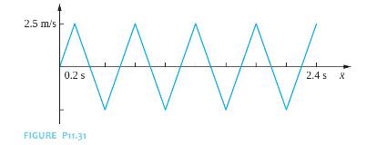
Use the finite-element model of Chapter Problem 11.30 to determine the response of the structure if it is subject to the earthquake of Figure P11.31.Data From Chapter Problem 11.31: 2.5 m/s 0.2 s FIGURE P11.31 2.45 x
Use the finite-element model of Chapter Problem 11.30 to determine the response of the structure if HVAC equipment on the girder produces a lateral harmonic force of magnitude \(3000 \mathrm{~N}\) at a frequency of \(500 \mathrm{rpm}\).Data From Chapter Problem 11.30: 2.5 m FIGURE P11.30 5.1 m 2000
Use two bar elements to model each member of the truss of Example 11.12 and approximate the three lowest natural frequencies of the truss.Example 11.12:Use the finite-element method to approximate the lowest natural frequency for the truss of Figure 11.16(a). Use one bar element for each truss
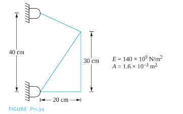
Use one bar element to model each member of the truss of Figure P11.34 and approximate its two lowest natural frequencies. b 40 cm FIGURE P11.34 -20 cm 30 cm E 140 x 109 N/m A = 1.6 10-3 m
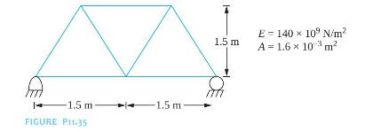
Use one bar element to model each member of the truss of Figure P11.35 and approximate its two lowest natural frequencies. 1.5 m 1.5 m- FIGURE P11.35 1.5 m E-140 x 109 N/m A = 1.6 103 m
A beam is placed on an elastic foundation whose stiffness per unit length is \(k\). Derive the element \(k_{23}\) of the local stiffness matrix for a beam element of length \(l\) including the stiffness of the elastic foundation.
A beam is subject to a constant axial load of magnitude \(P\), which is applied along the beam's neutral axis. Derive the element \(k_{31}\) of the local stiffness matrix for a beam element of length \(l\), including the effect of transverse displacement due to the axial load.
A beam is rotating about an axis with an angular velocity \(\omega\). Determine the element \(m_{13}\) of the local mass matrix for a beam element of length \(l\), including the kinetic energy due to the rotation of the beam. The left end of the element is a distance \(r\) from the axis of rotation.
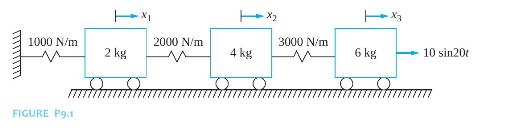
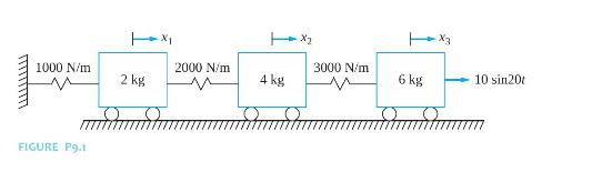
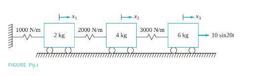
Determine the steady-state amplitudes of vibration of each of the masses of the system in Figure P9.1. Use the method of undetermined coefficients. X2 X3 1000 N/m 2000 N/m 3000 N/m 2 kg 4 kg 6 kg 10 sin20 www FIGURE P9.1
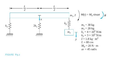
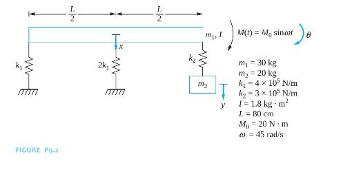
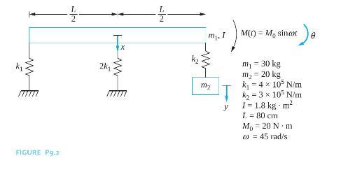
Determine the steady-state amplitude for the mass hanging from the end of the bar in the system in Figure P9.2. Use the method of undetermined coefficients. FIGURE P9.2 L 2 2k1 W m, I M(t) = M sincot X m2 y m = 30 kg m = 20 kg k = 4 105 N/m k = 3 105 N/m I=1.8 kg-m I. 80 cm Mo 20 N m 0 = 45 rad/s
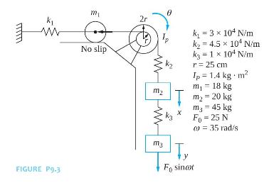
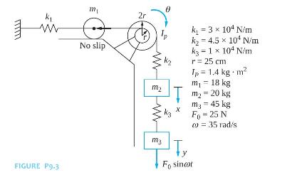
Determine the steady-state amplitude of vibration of the mass \(m_{3}\) of the system in Figure P9.3. Use the method of undetermined coefficients. k mi w No slip FIGURE P9.3 2r w m W m3 k = 3 104 N/m k = 4.5 10 N/m k3 - 1 x 104 N/m r = 25 cm Ip=1.4 kg. m m = 18 kg m = 20 kg m3 = 45 kg Fo=25 N =35
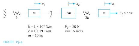
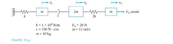
Determine the steady-state amplitudes of vibration of each of the masses of the system in Figure P9.4. Use the method of undetermined coefficients. x X2 2m ww m Fo sincor 2k w k m k = 1 10+ N/m F = 20 N c 100 N s/m 0 - 15 rad/s m = 10 kg FIGURE P9.4
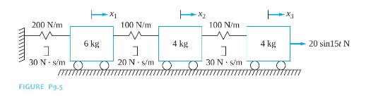
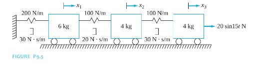
Determine the steady-state amplitudes of vibration of each of the masses of the system in Figure P9.5. Use the method of undetermined coefficients. 200 N/m ] 30 N s/m FIGURE P9.5 X1 100 N/m -X2 100 N/m x3 6 kg 4 kg 4 kg 20 sin15t N ] 20 N s/m 30 N s/m
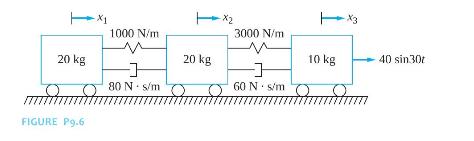
Determine the steady-state amplitudes of vibration of each of the masses of the system in Figure P9.6. Use the method of undetermined coefficients. 20 kg FIGURE P9.6 1000 N/m 1 80 N s/m O 3000 N/m -X3 20 kg 10 kg 40 sin 30t 1 60 N s/m
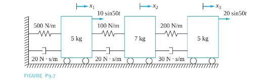
Determine the steady-state responses of each of the masses of the system in Figure P9.7. Use the method of undetermined coefficients. 500 N/m w 20 N s/m FIGURE P9.7 5 kg X1 10 sin50t 100 N/m 200 N/m w w 7 kg 5 kg 20 N s/m O 30 Ns/m X3 20 sin50t
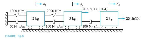
Determine the steady-state responses of each of the masses of the system in Figure P9.8. Use the method of undetermined coefficients. 1000 N/m 50 N s/m FIGURE P9.8 20 sin(30t+/4) X3 2000 N/m 2 kg 3 kg 2 kg 20 sin30r 100 N s/m 100 N s/m
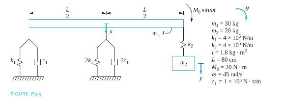
Determine the steady-state response of the hanging mass in the system of Figure P9.9. Use the method of undetermined coefficients. FIGURE P9.9 L 2 2k X 201 L Mo sincot 2 m2 m = 30 kg m = 20 kg k = 4 105 N/m k = 4 10 N/m 1- 1.8 kg + m L= 80 cm T M = 20 Nm @ = 45 rad/s y c =1 x 103 N s/m
Determine the steady-state amplitudes of vibration of each of the masses in the system of Figure P9.1. Use the Laplace transform method. X3 1000 N/m 2000 N/m 3000 N/m 2 kg 4 kg 6 kg 10 sin20 FIGURE P9.1 0
Determine the steady-state amplitudes of vibration of the hanging mass in the system of Figure P9.2. Use the Laplace transform method. ww FIGURE P9.2 12 2k1 WW 72 X k WW m2 M(t) = Mosinoor 1) e m = 30 kg m = 20 kg k = 4 105 N/m y k2-3 105 N/m I = 1.8 kg m I. 80 cm M = 20 N m 0 = 45 rad/s
Determine the steady-state amplitude of vibration of the mass \(m_{3}\) of the system in Figure P9.3. Use the Laplace transform method. w FIGURE P9-3 m No slip 2r w m W mz T k 3 x 10 N/m k = 4.5 104 N/m k3 - 1 x 104 N/m r = 25 cm Tp = 1.4 kg-m m = 18 kg m = 20 kg m3 - 45 kg Fo=25 N 0 = 35 rad/s Fo
Determine the steady-state amplitudes of vibration of each of the masses of the system in Figure P9.4. Use the Laplace transform method. w k FIGURE P9-4 m k = 1 10+ N/m x c 100 N s/m m = 10 kg X2 2m w Fo-20 N @ 15 rad/s 2k m x3 Fo sinot
Determine the steady-state amplitudes of vibration of each of the masses of the system in Figure P9.5. Use the Laplace transform method. 200 N/m ] 30 N s/m FIGURE P9.5 100 N/m X2 100 N/m X3 6 kg 4 kg 4 kg 20 sin15t N ] 20 N s/m ] 30 N s/m
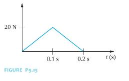
Determine the response of the \(2 \mathrm{~kg}\) mass of Figure P9. 1 if the sinusoidal force is replaced by the triangular pulse of Figure P9.15. Use the Laplace transform method. 20 N FIGURE P9.15 0.1 s 0.2 s 1(s)
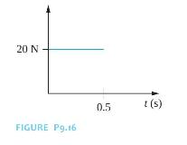
Determine the response of the \(6 \mathrm{~kg}\) mass of Figure P9.1 if the sinusoidal force is replaced by the rectangular pulse of Figure P9.16. Use the Laplace transform method. 20 N FIGURE P9.16 0.5 t(s)
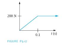
Determine the response of the system of Figure P9.2 if the sinusoidal force is replaced by the force of Figure P9.17. Use the Laplace transform method. 200 N FIGURE P9.17 + 0.1 t(s)
Repeat Chapter Problem 9.1 using modal analysis.Data From Chapter Problem 9.1: Determine the steady-state amplitudes of vibration of each of the masses of the system in Figure P9.1. Use the method of undetermined coefficients. X2 X3 1000 N/m 2000 N/m 3000 N/m 2 kg 4 kg 6 kg 10 sin20 www FIGURE P9.1
Repeat Chapter Problem 9.2 using modal analysis.Data From Chapter Problem 9.2:Determine the steady-state amplitude for the mass hanging from the end of the bar in the system in Figure P9.2. Use the method of undetermined coefficients. FIGURE P9.2 L 2 2k1 W m, I M(t) = M sincot X m2 y m = 30 kg m =
Repeat Chapter Problem 9.3 using modal analysis.Data From Chapter Problem 9.3:Determine the steady-state amplitude of vibration of the mass \(m_{3}\) of the system in Figure P9.3. Use the method of undetermined coefficients. k mi w No slip FIGURE P9.3 2r w m W m3 k = 3 104 N/m k = 4.5 10 N/m k3 -
Repeat Chapter Problem 9.15 using modal analysisData From Chapter Problem 9.15:Determine the response of the \(2 \mathrm{~kg}\) mass of Figure P9. 1 if the sinusoidal force is replaced by the triangular pulse of Figure P9.15. Use the Laplace transform method. 20 N FIGURE P9.15 0.1 s 0.2 s 1(s)
Repeat Chapter Problem 9.16 using modal analysis.Data From Chapter Problem 9.16:Determine the response of the \(6 \mathrm{~kg}\) mass of Figure P9.1 if the sinusoidal force is replaced by the rectangular pulse of Figure P9.16. Use the Laplace transform method. 20 N FIGURE P9.16 0.5 t(s)
Repeat Chapter Problem 9.7 using modal analysis.Data From Chapter Problem 9.7:Determine the steady-state responses of each of the masses of the system in Figure P9.7. Use the method of undetermined coefficients. 500 N/m w 20 N s/m FIGURE P9.7 5 kg X1 10 sin50t 100 N/m 200 N/m w w 7 kg 5 kg 20 N s/m
Repeat Chapter Problem 9.9 using modal analysis.Data From Chapter Problem 9.8:Determine the steady-state response of the hanging mass in the system of Figure P9.9. Use the method of undetermined coefficients. FIGURE P9.9 L 2 2k X 201 L Mo sincot 2 m2 m = 30 kg m = 20 kg k = 4 105 N/m k = 4 10 N/m
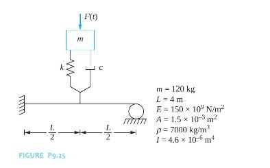
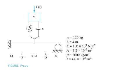
Figure P9.25 shows a machine attached to a fixed-pinned beam through an isolator. Design an isolator of damping ratio 0.1 such that the force transmitted to the beam is \(2000 \mathrm{~N}\) when the machine is subject to a harmonic excitation with an amplitude of \(12,000 \mathrm{~N}\) at a
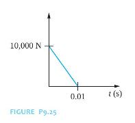
Design an isolator with a damping ratio of 0.4 for the system of Figure P9.25 when it is subject to the pulse of Figure P9.26. The maximum force transmitted to the beam should be \(500 \mathrm{~N}\). 10,000 N. FIGURE P9.25 0.01 t(s)
A continuous system is also referred to as a distributed parameter system.Indicate whether the statement presented is true or false. If true, state why. If false, rewrite the statement to make it true.
A continuous system has an infinite number of natural frequencies.Indicate whether the statement presented is true or false. If true, state why. If false, rewrite the statement to make it true.
The longitudinal vibrations of a bar and the transverse vibrations of a beam are both governed by the wave equation.Indicate whether the statement presented is true or false. If true, state why. If false, rewrite the statement to make it true.
A free-free beam is an example of a degenerate system.Indicate whether the statement presented is true or false. If true, state why. If false, rewrite the statement to make it true.
Rayleigh's quotient defined for a system is stationary for any function that satisfies the boundary conditions of that system.Indicate whether the statement presented is true or false. If true, state why. If false, rewrite the statement to make it true.
Four initial conditions are necessary to determine the forced-vibration response of a fixed-free beam.Indicate whether the statement presented is true or false. If true, state why. If false, rewrite the statement to make it true.
The Rayleigh-Ritz method can be used to approximate natural frequencies and forced responses of continuous systems.Indicate whether the statement presented is true or false. If true, state why. If false, rewrite the statement to make it true.
Mode shapes corresponding to distinct natural frequencies of a continuous system are orthogonal with respect to the potential-energy scalar product.Indicate whether the statement presented is true or false. If true, state why. If false, rewrite the statement to make it true.
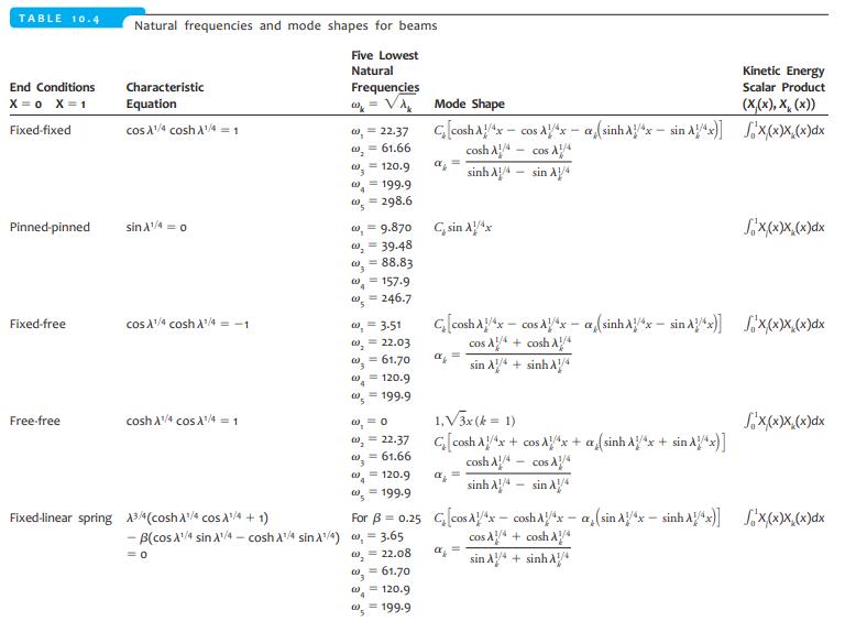
The mode shape reported in Table 10.4 for a pinned-free beam of \(\sqrt{3} x\) is a rigid-body mode.Indicate whether the statement presented is true or false. If true, state why. If false, rewrite the statement to make it true. TABLE 10.4 End Conditions X=0 X=1 Fixed-fixed Natural frequencies and
The assumption that \(M=-E I \frac{\partial^{2} w}{\partial x^{2}}\) is used in the derivation of the differential equation governing the transverse vibrations of a beam.Indicate whether the statement presented is true or false. If true, state why. If false, rewrite the statement to make it true.
What is the method where a product solution is assumed for the free vibrations of a uniform bar called? Is the same method applicable to the free vibrations of a beam?
What is the order of the highest spatial derivative in the wave equation? What is the order of the highest spatial derivative of the beam equation?
What is the process of introducing the independent variables \(t^{*}\) and \(x^{*}\) and the dependent variable \(w^{*}\) called?
How many boundary conditions are required to determine the response of(a) A beam undergoing transverse vibrations?(b) A bar undergoing longitudinal vibrations?(c) A shaft undergoing torsional oscillations?
What does the boundary condition \(\frac{\partial \theta}{\partial x}(L, t)\) mean physically when applied to a torsional shaft.
What are the boundary conditions for the free vibrations of a longitudinal bar fixed at \(x=0\) and free at \(x=L\) ?
What are the boundary conditions for the free vibrations of a torsional shaft fixed at \(x=0\) and attached to a thin disk with a mass moment of inertia \(I\) at \(x=L\) ?
What are the boundary conditions for the free vibrations of a torsional shaft free at \(x=0\) and attached to a thin disk with a mass moment of inertia \(I\) and a torsional spring of stiffness \(k_{t}\) at \(x=L\) ?
What are the boundary conditions for the free vibrations of a string fixed at \(x=0\) and attached to a spring of stiffness \(k\) at \(x=L\) ?

Showing 500 - 600 of 4547

1
2
3
4
5
6
7
8
9
10
11
12
13
14
15
Last

Step by Step Answers

Services

Sitemap
Fun
Definitions
Become Tutor
Used Textbooks
Study Help Categories
Recent Questions
Expert Questions
Campus Wear
Sell Your Books

Company Info

Security
Copyrights
Privacy Policy
Terms & Conditions
SolutionInn Fee
Scholarship
Online Quiz
Give Feedback, Get Rewards

Get In Touch

About Us
Contact Us
Career
Jobs
FAQ
Student Discount
Campus Ambassador

Secure Payment

Download Our App

© 2026 SolutionInn. All Rights Reserved