New Semester Started Get 50% OFF Study Help! --h --m --s Claim Now

Question Answers

Textbooks

Find textbooks, questions and answers

Oops, something went wrong!

Change your search query and then try again

Result Not Found

Books FREE
Study Help
Tutors
AI Study Planner NEW
Sell Books

Search
Sign In
Register

study help
engineering
introduction mechanical engineering

Mechanical Vibrations Theory And Applications 1st Edition S. GRAHAM KELLY - Solutions

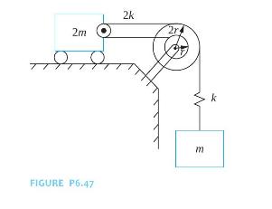
Determine the natural frequencies and modal fractions for the two degree-offreedom system of Figure P6.47. 2m 2k 2r: FIGURE P6.47 m k
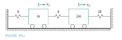
Determine the frequency response of the system of Figure P6.1 and Chapter Problem 6.10 due to a sinusoidal force \(F_{0} \sin \omega t\) applied to the block whose displacement is \(x_{1}\).Data From Chapter Problem 6.10:Determine the natural frequencies of the system of Figure P6.1 if \(m=10
Determine the frequency response of the system of Figure P6.1 and Chapter Problem 6.10 due to a sinusoidal force \(F_{0} \sin \omega t\) applied to the block whose displacement is \(x_{2}\).Data From Chapter Problem 6.10:Determine the natural frequencies of the system of Figure P6.1 if \(m=10
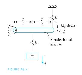
Determine the frequency response of the system of Figure P6.2 and Chapter Problem 6.11 due to a sinusoidal force \(F_{0} \sin \omega t\) applied to the particle.Data From Chapter Problem 6.11:Determine the natural frequencies of the system of Figure P6.2 if \(m=2 \mathrm{~kg}\), \(L=1 \mathrm{~m}\)
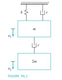
Determine the frequency response of the system of Figure P6.7 and Chapter Problem 6.42 due to a sinusoidal force \(F_{0} \sin \omega t\) applied to the block whose displacement is \(x_{1}\).Data From Chapter Problem 6.42:Determine the response of the system of Figure 6.7 due to a force \(F(t)=\)
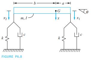
Determine the frequency response of the system of Figure P6.8 and Chapter Problem 6.43 due to a sinusoidal force \(F_{0} \sin \omega t\) applied to the mass center of the machine tool.Data From Chapter Problem 6.43:Determine the response of the system of Figure P6.8 due to a unit impulse applied at
Determine the frequency response of the system of Figure P6.8 and Chapter Problem 6.43 due to a sinusoidal force \(F_{0} \sin \omega t\) applied to the right end of the machine tool.Data From Chapter Problem 6.43:Determine the response of the system of Figure P6.8 due to a unit impulse applied at
A \(50 \mathrm{~kg}\) lathe mounted on an elastic foundation of stiffness \(4 \times 10^{5} \mathrm{~N} / \mathrm{m}\) has a vibration amplitude of \(35 \mathrm{~cm}\) when the motor speed is \(95 \mathrm{rad} / \mathrm{s}\). Design an undamped dynamic vibration absorber such that steady-state
What is the required stiffness of an undamped dynamic vibration absorber whose mass is \(5 \mathrm{~kg}\) to eliminate vibrations of a \(25 \mathrm{~kg}\) machine of natural frequency \(125 \mathrm{rad} / \mathrm{s}\) when the machine operates at \(110 \mathrm{rad} / \mathrm{s}\) ?
A \(35 \mathrm{~kg}\) machine is attached to the end of a cantilever beam of length \(2 \mathrm{~m}\), elastic modulus \(210 \times 10^{9} \mathrm{~N} / \mathrm{m}^{2}\), and moment of inertia \(1.3 \times 10^{-7} \mathrm{~m}^{4}\). The machine operates at \(180 \mathrm{rpm}\) and has a rotating
A \(150 \mathrm{~kg}\) pump experiences large-amplitude vibrations when operating at \(1500 \mathrm{rpm}\). Assuming this is the natural frequency of a SDOF system, design a dynamic vibration absorber such that the lower natural frequency of the two degree-of-freedom system is less than \(1300
A solid disk of diameter \(30 \mathrm{~cm}\) and mass \(10 \mathrm{~kg}\) is attached to the end of a solid 3-cm-diameter, 1-m-long steel shaft \(\left(G=80 \times 10^{9} \mathrm{~N} / \mathrm{m}^{2}\right)\). A torsional vibration absorber consists of a disk attached to a shaft that is then
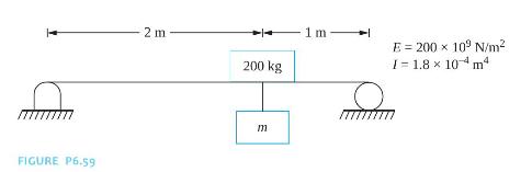
A \(200 \mathrm{~kg}\) machine is placed on a massless simply supported beam as shown in Figure P6.59. The machine has a rotating unbalance of \(1.41 \mathrm{~kg} \cdot \mathrm{m}\) and operates at \(3000 \mathrm{rpm}\). The steady-state vibrations of the machine are to be absorbed by hanging a
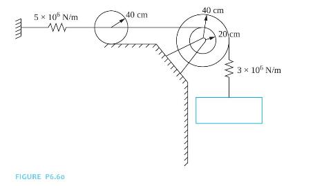
The disk in Figure P6.60 rolls without slip and the pulley is massless. What is the mass of the block that should be hung from the cable such that steady-state vibrations of the cylinder are eliminated when \(\omega=120 \mathrm{rad} / \mathrm{s}\) ? www 5 x 106 N/m w 40 cm FIGURE P6.60 40 cm 20 cm
Vibration absorbers are used in boxcars to protect sensitive cargo from large accelerations due to periodic excitations provided by rail joints. For a particular railway, joints are spaced \(5 \mathrm{~m}\) apart. The boxcar, when empty, has a mass of \(25,000 \mathrm{~kg}\). Two absorbers, each of
A \(500 \mathrm{~kg}\) reciprocating machine is mounted on a foundation of equivalent stiffness \(5 \times 10^{6} \mathrm{~N} / \mathrm{m}\). When operating at \(800 \mathrm{rpm}\), the machine produces an unbalanced harmonic force of magnitude \(50,000 \mathrm{~N}\). Two cantilever beams with end
A \(100 \mathrm{~kg}\) machine is placed at the midspan of a 2-m-long cantilever beam \(\left(E=210 \times 10^{9} \mathrm{~N} / \mathrm{m}^{2}, I=2.3 \times 10^{-6} \mathrm{~m}^{4}\right)\). The machine produces a harmonic force of amplitude 60,000 N. Design a damped vibration absorber of mass \(30
Repeat Chapter Problem 6.63 if the excitation is due to a rotating unbalance of magnitude \(0.33 \mathrm{~kg} \cdot \mathrm{m}\).Data From Chapter Problem 6.63:A \(100 \mathrm{~kg}\) machine is placed at the midspan of a 2-m-long cantilever beam \(\left(E=210 \times 10^{9} \mathrm{~N} /
For the absorber designed in Chapter Problem 6.63, what is the minimum steady-state amplitude of the machine and at what speed does it occur?Data From Chapter Problem 6.63:A \(100 \mathrm{~kg}\) machine is placed at the midspan of a 2-m-long cantilever beam \(\left(E=210 \times 10^{9} \mathrm{~N} /
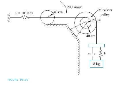
Determine values of \(k\) and \(c\) such that the steady-state amplitude of the center of the cylinder in Figure \(\mathrm{P} 6.66\) is less than \(4 \mathrm{~mm}\) for \(60 \mathrm{rad} / \mathrm{s} 5 105 N/m ww 40 cm FIGURE P6.66 200 sinet LL Massless pulley 20 cm 40 cm 8 kg W
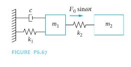
Use the Laplace transform method to analyze the situation of an undamped absorber attached to a viscously damped system, as shown in Figure P6.67.(a) Determine the steady-state amplitude of the mass \(m_{1}\).(b) Use the results of part (a) to design an absorber for a \(123 \mathrm{~kg}\) machine
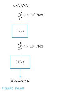
Design an undamped absorber such that the steady-state motion of the \(25 \mathrm{~kg}\) machine component in Figure P6.68 ceases when the absorber is added. What is the steady-state amplitude of the \(31 \mathrm{~kg}\) component? 5 x 10 N/m 25 kg 4 x 104 N/m 31 kg 200sin67t N FIGURE P6.68
A \(300 \mathrm{~kg}\) compressor is placed at the end of a cantilever beam of length \(1.8 \mathrm{~m}\), elastic modulus \(200 \times 10^{9} \mathrm{~N} / \mathrm{m}^{2}\), and moment of inertia \(1.8 \times 10^{-5} \mathrm{~m}^{4}\). When the compressor operates at \(1000 \mathrm{rpm}\), it has
An engine has a moment of inertia of \(7.5 \mathrm{~kg} \cdot \mathrm{m}^{2}\) and a natural frequency of \(125 \mathrm{~Hz}\). Design a Houdaille damper such that the engine's maximum magnification factor is 4.8. During operation, the engine is subject to a harmonic torque of magnitude \(150
A \(200 \mathrm{~kg}\) machine is subjected to an excitation of magnitude \(1500 \mathrm{~N}\). The machine is mounted on a foundation of stiffness \(2.8 \times 10^{6} \mathrm{~N} / \mathrm{m}\). What are the mass and damping coefficient of an optimally designed vibration damper such that the
The differential equations for a linear MDOF system can be written in a matrix form.Indicate whether the statement presented is true or false. If true, state why. If false, rewrite the statement to make it true.
Lagrange's equations can be used to derive the differential equations governing the motion only for linear systems.Indicate whether the statement presented is true or false. If true, state why. If false, rewrite the statement to make it true.
Lagrange's equations can be used for conservative systems and nonconservative systems.Indicate whether the statement presented is true or false. If true, state why. If false, rewrite the statement to make it true.
The FBD method, when applied to a MDOF linear system, always leads to symmetric mass, stiffness, and damping matrices.Indicate whether the statement presented is true or false. If true, state why. If false, rewrite the statement to make it true.
Lagrange's equations, when applied to a MDOF linear system, always leads to symmetric mass, stiffness, and damping matrices.Indicate whether the statement presented is true or false. If true, state why. If false, rewrite the statement to make it true.
The quadratic form of the potential energy can be used to determine the stiffness matrix for a linear MDOF system.Indicate whether the statement presented is true or false. If true, state why. If false, rewrite the statement to make it true.
A system is dynamically coupled if the mass matrix for the system is not symmetric.Indicate whether the statement presented is true or false. If true, state why. If false, rewrite the statement to make it true.
The choice of generalized coordinates is irrelevant in deciding whether a system is dynamically coupled.Indicate whether the statement presented is true or false. If true, state why. If false, rewrite the statement to make it true.
The flexibility matrix is the transpose of the stiffness matrix.Indicate whether the statement presented is true or false. If true, state why. If false, rewrite the statement to make it true.
A diagonal stiffness matrix means that \(k_{i j}=k_{i j}\) for all \(i, j=1,2, \ldots, n\).Indicate whether the statement presented is true or false. If true, state why. If false, rewrite the statement to make it true.
Elements of the mass matrix for a MDOF system may have different dimensions.Indicate whether the statement presented is true or false. If true, state why. If false, rewrite the statement to make it true.
The formulation of the stiffness influence coefficient method to determine the stiffness matrix for a linear MDOF system relies on the concept that potential energy is a function of position.Indicate whether the statement presented is true or false. If true, state why. If false, rewrite the
When flexibility influence coefficients are used to calculate the flexibility matrix for a MDOF system, the flexibility matrix is calculated one column at a time.Indicate whether the statement presented is true or false. If true, state why. If false, rewrite the statement to make it true.
The stiffness matrix for a system always exists but the flexibility matrix does not always exist.Indicate whether the statement presented is true or false. If true, state why. If false, rewrite the statement to make it true.
A system is not statically coupled if its flexibility matrix is a diagonal matrix.Indicate whether the statement presented is true or false. If true, state why. If false, rewrite the statement to make it true.
Lagrange's equations can be used to derive the equations governing the vibrations of three masses along the span of a beam ignoring the inertia of the beam and using three degrees of freedom in the model.Indicate whether the statement presented is true or false. If true, state why. If false,
Write the general matrix form of the differential equations governing the undamped and forced vibrations of a linear \(n\) DOF system.
State Lagrange's equations for a conservative system.
What defines whether a system is dynamically coupled?
How is Rayleigh's dissipation function used?
What is a variation?
How is the method of virtual work applied in the application of Lagrange's equations for a MDOF system?
What is Maxwell's reciprocity relation and how is it applied?
Write the differential equations governing a MDOF system in matrix form when the mass matrix, damping matrix, and flexibility matrix are known.
Describe the calculation of the stiffness influence coefficient \(k_{13}\).The generalized coordinates for modeling a system have been selected as \(x_{1}, x_{2}\), and \(\theta\) where \(x_{1}\) and \(x_{2}\) are linear displacements and \(\theta\) is an angular coordinate.
Describe the calculation of the flexibility influence coefficient \(a_{13}\).The generalized coordinates for modeling a system have been selected as \(x_{1}, x_{2}\), and \(\theta\) where \(x_{1}\) and \(x_{2}\) are linear displacements and \(\theta\) is an angular coordinate.
Describe the calculation of the inertia influence coefficient \(m_{12}\).The generalized coordinates for modeling a system have been selected as \(x_{1}, x_{2}\), and \(\theta\) where \(x_{1}\) and \(x_{2}\) are linear displacements and \(\theta\) is an angular coordinate.
Describe the calculation of the inertia influence coefficient \(m_{31}\).The generalized coordinates for modeling a system have been selected as \(x_{1}, x_{2}\), and \(\theta\) where \(x_{1}\) and \(x_{2}\) are linear displacements and \(\theta\) is an angular coordinate.
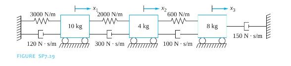
What is the kinetic energy of the system of Figure SP7.29 at an arbitrary instant? 3000 N/m ww ] 10 kg x 2000 N/m www C 120 N. s/mm/300 N. s/m FIGURE SP7.29 4 kg 600 N/m ww E 8 kg 1100 N. s/mmmmmmm 150 N s/m
What is the potential energy in the system of Figure SP7.29 at an arbitrary instant? 3000 N/m www + 120 N s/m FIGURE SP7:29 2000 N/m ww 10 kg 4 kg ++ 300 N s/m 600 N/m ww +- 100 Ns/m 8 kg 150 N s/m
What is Rayleigh's dissipation function for the system of Figure SP7.29 at an arbitrary instant? 3000 N/m + 120 N s/m FIGURE SP7:29 10 kg 2000 N/m www + 300 N s/m 4 kg 600 N/m ww +- 100 N-s/m 8 kg 150 N s/m
What is the result of\[ \frac{d}{d t}\left[\frac{\partial}{\partial \dot{x}}(2 \dot{x}-\dot{y})^{2}\right] \]
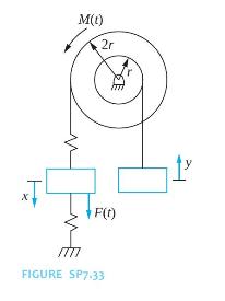
What is virtual work done by the external forces in Figure SP7.33, assuming virtual displacements \(\delta x\) and \(\delta y\) ? M(t) 2r F(t) FIGURE SP7.33
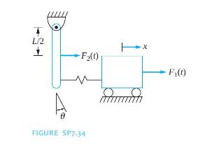
What are the generalized forces for the system of Figure SP7.34 using \(x\) and \(\theta\) as generalized coordinates? L/2 1 -x -F2(t) A FIGURE SP7.34 F(t)
The quadratic form of the potential energy for a three degree-of-freedom system is\[ V=5 x_{1}^{2}+4 x_{1} x_{2}+2 x_{1} x_{3}+8 x_{2}^{2}+3 x_{2} x_{2}+6 x_{3}^{2} \]Determine the stiffness matrix for the system.
The kinetic energy for a three degree-of-freedom system is\[ T=3\left(\dot{x}_{2}-\frac{1}{2} \dot{x}_{1}\right)^{2}+12\left(\dot{x}_{2}+\frac{1}{3} \dot{x}_{1}\right)^{2}+4 \dot{x}_{3}^{2} \]Determine the mass matrix for the system.
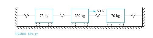
When a load of \(50 \mathrm{~N}\) is applied to the \(250 \mathrm{~kg}\) mass in the system of Figure SP7.37, the displacements of the masses are \(x_{1}=3 \mathrm{~mm}, x_{2}=5 \mathrm{~mm}\), and \(x_{3}=2.5 \mathrm{~mm}\). Determine all possible elements of the system's flexibility matrix.
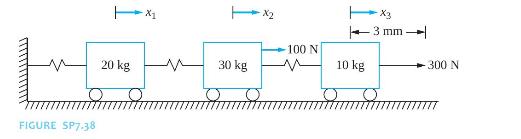
When the block of mass \(10 \mathrm{~kg}\) is given a displacement of \(3 \mathrm{~mm}\) in the system of Figure SP7.38 and all other blocks are held in their equilibrium positions, it is found that the forces on the blocks are \(F_{1}=0, F_{2}=100 \mathrm{~N}\), and \(F_{3}=300 \mathrm{~N}\).
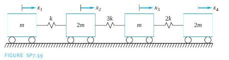
What is the determinant of the stiffness matrix of the system of Figure SP7.39? m FIGURE SP7.39 k 2m X 3k -X3 2k H m 2m X4
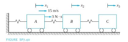
When block \(A\) of Figure SP7. 40 is given a velocity of \(15 \mathrm{~m} / \mathrm{s}\) and the velocities of blocks \(B\) and \(C\) remain at rest, an impulse of \(3 \mathrm{~N} \cdot \mathrm{s}\) applied to block \(A\) is required. Determine all possible elements of the system's mass matrix.
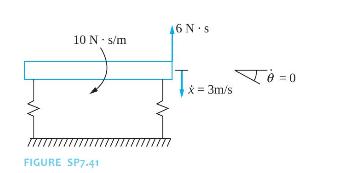
When the right end of the bar of the system of Figure SP7.41 is given a velocity of \(3 \mathrm{~m} / \mathrm{s}\) but the angular velocity of the bar is zero, an impulse of magnitude \(6 \mathrm{~N} \cdot \mathrm{s}\) is required at the right end of the bar and an angular impulse of \(10
Lagrange's equations are used to derive the differential equations for a three degree-of-freedom system resulting in\[ \left[\begin{array}{lll} m_{11} & m_{12} & m_{13} \\ m_{21} & m_{22} & m_{23} \\ m_{31} & m_{32} & m_{33} \end{array}\right]\left[\begin{array}{c} \ddot{x}_{1} \\ \ddot{x}_{2} \\
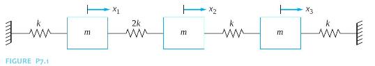
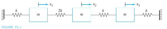
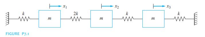
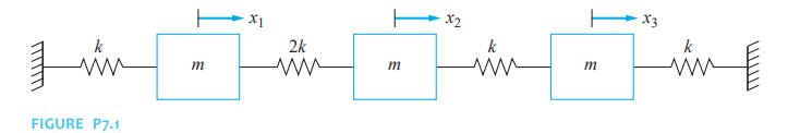
Use the free-body diagram method to derive the differential equations governing the motion of the systems shown in Figure P7.1 using the indicated generalized coordinates. Make linearizing assumptions and write the resulting equations in matrix form. k ww FIGURE P7.1 2k k m ww m ww m X3. k
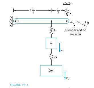
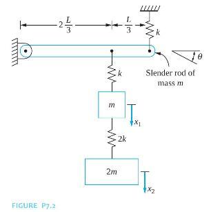
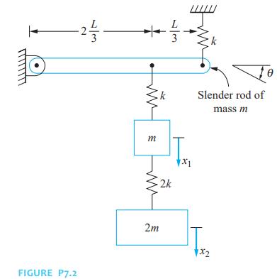
Use the free-body diagram method to derive the differential equations governing the motion of the systems shown in Figure P7.2 using the indicated generalized coordinates. Make linearizing assumptions and write the resulting equations in matrix form. -21- FIGURE P7.2 k Slender rod of mass m m x 2k
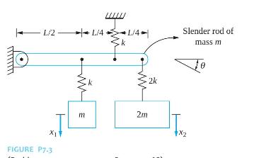
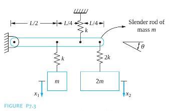
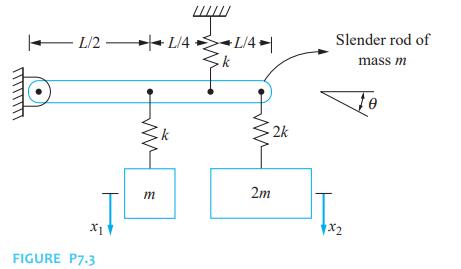
Use the free-body diagram method to derive the differential equations governing the motion of the systems shown in Figure P7.3 using the indicated generalized coordinates. Make linearizing assumptions and write the resulting equations in matrix form. 1/2 | 1/4 - L/4 L/4 -k FIGURE P7-3 E 2k Slender
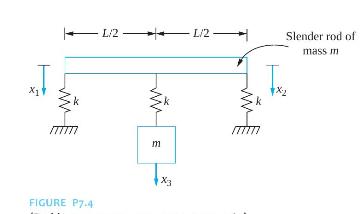
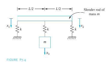
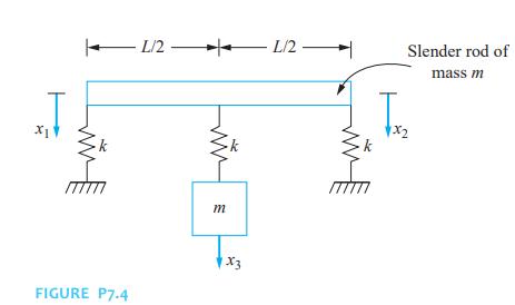
Use the free-body diagram method to derive the differential equations governing the motion of the systems shown in Figure P7.4 using the indicated generalized coordinates. Make linearizing assumptions and write the resulting equations in matrix form. X1 L/2 L/2- Slender rod of mass m m FIGURE P7-4
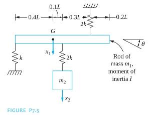
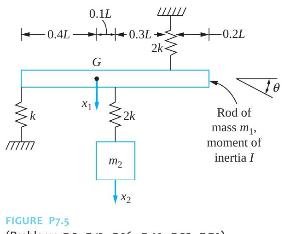
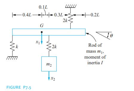
Use the free-body diagram method to derive the differential equations governing the motion of the systems shown in Figure P7.5 using the indicated generalized coordinates. Make linearizing assumptions and write the resulting equations in matrix form. 0.1L 0.41 0.31 G 2k -0.2L x1 m2 FIGURE P7.5 1X2
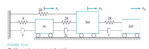
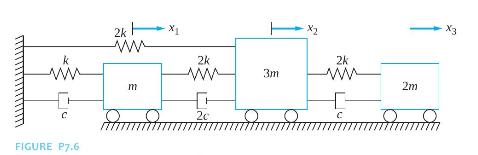
Use the free-body diagram method to derive the differential equations governing the motion of the systems shown in Figure P7.6 using the indicated generalized coordinates. Make linearizing assumptions and write the resulting equations in matrix form. k ww 2k H www C FIGURE P7.6 2k 2k ww 3m www m 2m
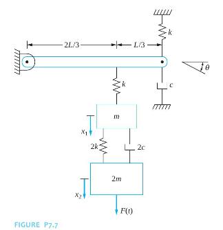
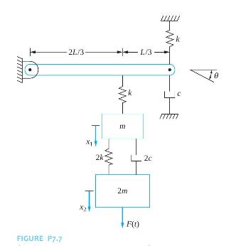
Use the free-body diagram method to derive the differential equations governing the motion of the systems shown in Figure P7.7 using the indicated generalized coordinates. Make linearizing assumptions and write the resulting equations in matrix form. 2L/3- FIGURE P7.7 X1 X21 WE L/3 uyu k 2k 2c 2m
Use Lagrange's equations to derive the differential equations governing the motion of the systems shown in Figures P7.1. Use the indicated generalized coordinates. Make linearizing assumptions, and write the resulting equations in matrix form. Indicate whether the system is statically coupled,
Use Lagrange's equations to derive the differential equations governing the motion of the systems shown in Figures P7.2. Use the indicated generalized coordinates. Make linearizing assumptions, and write the resulting equations in matrix form. Indicate whether the system is statically coupled,
Use Lagrange's equations to derive the differential equations governing the motion of the systems shown in Figures P7.3. Use the indicated generalized coordinates. Make linearizing assumptions, and write the resulting equations in matrix form. Indicate whether the system is statically coupled,
Use Lagrange's equations to derive the differential equations governing the motion of the systems shown in Figures P7.4. Use the indicated generalized coordinates. Make linearizing assumptions, and write the resulting equations in matrix form. Indicate whether the system is statically coupled,
Use Lagrange's equations to derive the differential equations governing the motion of the systems shown in Figures P7.5. Use the indicated generalized coordinates. Make linearizing assumptions, and write the resulting equations in matrix form. Indicate whether the system is statically coupled,
Use Lagrange's equations to derive the differential equations governing the motion of the systems shown in Figures P7.6. Use the indicated generalized coordinates. Make linearizing assumptions, and write the resulting equations in matrix form. Indicate whether the system is statically coupled,
Use Lagrange's equations to derive the differential equations governing the motion of the systems shown in Figures P7.7. Use the indicated generalized coordinates. Make linearizing assumptions, and write the resulting equations in matrix form. Indicate whether the system is statically coupled,
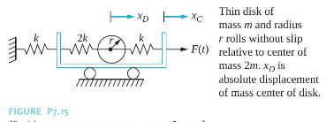
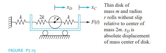
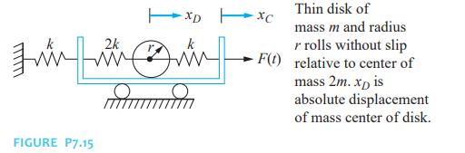
Use Lagrange's equations to drive the differential equations governing the motion of the systems shown in Figures P7.15. Use the indicated generalized coordinates. Make linearizing assumptions, and write the resulting equations in matrix form. Indicate whether the system is statically coupled,
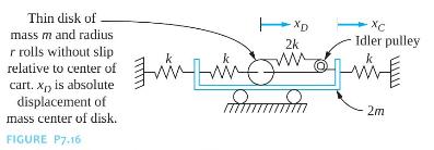
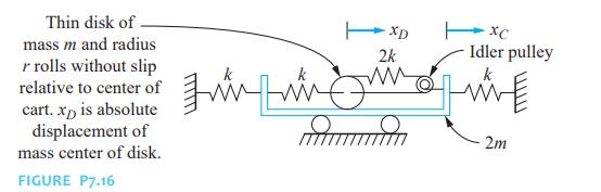
Use Lagrange's equations to drive the differential equations governing the motion of the systems shown in Figures P7.16. Use the indicated generalized coordinates. Make linearizing assumptions, and write the resulting equations in matrix form. Indicate whether the system is statically coupled,
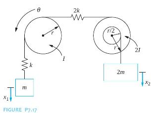
Use Lagrange's equations to drive the differential equations governing the motion of the systems shown in Figures P7.17. Use the indicated generalized coordinates. Make linearizing assumptions, and write the resulting equations in matrix form. Indicate whether the system is statically coupled,
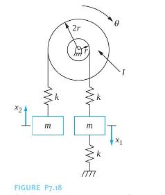
Use Lagrange's equations to drive the differential equations governing the motion of the systems shown in Figures P7.18. Use the indicated generalized coordinates. Make linearizing assumptions, and write the resulting equations in matrix form. Indicate whether the system is statically coupled,
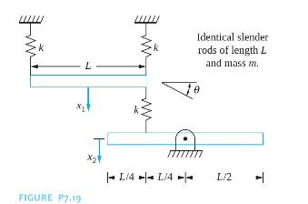
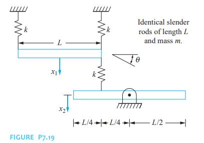
Use Lagrange's equations to drive the differential equations governing the motion of the systems shown in Figures P7.19. Use the indicated generalized coordinates. Make linearizing assumptions, and write the resulting equations in matrix form. Indicate whether the system is statically coupled,
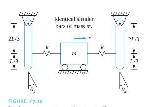
Use Lagrange's equations to drive the differential equations governing the motion of the systems shown in Figures P7.20. Use the indicated generalized coordinates. Make linearizing assumptions, and write the resulting equations in matrix form. Indicate whether the system is statically coupled,
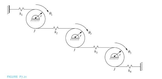
Use Lagrange's equations to drive the differential equations governing the motion of the systems shown in Figures P7.21. Use the indicated generalized coordinates. Make linearizing assumptions, and write the resulting equations in matrix form. Indicate whether the system is statically coupled,
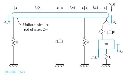
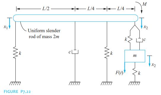
Use Lagrange's equations to drive the differential equations governing the motion of the systems shown in Figures P7.22. Use the indicated generalized coordinates. Make linearizing assumptions, and write the resulting equations in matrix form. Indicate whether the system is statically coupled,
Determine the kinetic energy of the system at an arbitrary instant for the systems of Figure P7.1. Put the kinetic energy in a quadratic form. Use the quadratic form to determine the mass matrix for the system. k www m FIGURE P7.1 -x1 2k www m X2 www m X3 k www
Determine the kinetic energy of the system at an arbitrary instant for the systems of Figure P7.3. Put the kinetic energy in a quadratic form. Use the quadratic form to determine the mass matrix for the system. L/2- L/2 L/4 x1 FIGURE P7.3 L/4 k 2k Slender rod of mass m Te m 2m 7x2
Determine the kinetic energy of the system at an arbitrary instant for the systems of Figure P7.4. Put the kinetic energy in a quadratic form. Use the quadratic form to determine the mass matrix for the system. L/2 -L/2- m FIGURE P7.4 X3 1x2 Slender rod of mass m
Determine the kinetic energy of the system at an arbitrary instant for the systems of Figure P7.5. Put the kinetic energy in a quadratic form. Use the quadratic form to determine the mass matrix for the system. 0.1L 0.4L 0.3L G www 2k- FIGURE P7.5 x1 2k m2 1x2 0.2L Rod of mass m, moment of inertia
Determine the kinetic energy of the system at an arbitrary instant for the systems of Figure P7.15. Put the kinetic energy in a quadratic form. Use the quadratic form to determine the mass matrix for the system. FIGURE P7.15 2k xDxC mum Thin disk of mass m and radius r rolls without slip F(t)
Determine the kinetic energy of the system at an arbitrary instant for the systems of Figure P7.19. Put the kinetic energy in a quadratic form. Use the quadratic form to determine the mass matrix for the system. FIGURE P7.19 X1 L X2 Identical slender rods of length L and mass m. | L/4 | L/4 | 1/2
Determine the kinetic energy of the system at an arbitrary instant for the systems of Figure P7.22. Put the kinetic energy in a quadratic form. Use the quadratic form to determine the mass matrix for the system. L/2 x1 Uniform slender rod of mass 2m www FIGURE P7.22 L/4 L/4 www 4 F(1) M x2 m Tx x2
Determine the potential energy of the system at an arbitrary instant for the systems of Figure P7.1. Put the potential energy in a quadratic form. Use the quadratic form to determine the stiffness matrix for the system. X2 k 2k ww m m k k m FIGURE P7.1
Determine the potential energy of the system at an arbitrary instant for the systems of Figure P7.2. Put the potential energy in a quadratic form. Use the quadratic form to determine the stiffness matrix for the system. FIGURE P7.2 L 23 k Slender rod of mass m m 2k 2m x2
Determine the potential energy of the system at an arbitrary instant for the systems of Figure P7.15. Put the potential energy in a quadratic form. Use the quadratic form to determine the stiffness matrix for the system. 2k FIGURE P7.15 xDxc mum Thin disk of mass m and radius r rolls without slip
Determine the potential energy of the system at an arbitrary instant for the systems of Figure P7.16. Put the potential energy in a quadratic form. Use the quadratic form to determine the stiffness matrix for the system. Thin disk of mass m and radius r rolls without slip relative to center of

Showing 900 - 1000 of 4547

First
3
4
5
6
7
8
9
10
11
12
13
14
15
16
17
Last

Step by Step Answers

Services

Sitemap
Fun
Definitions
Become Tutor
Used Textbooks
Study Help Categories
Recent Questions
Expert Questions
Campus Wear
Sell Your Books

Company Info

Security
Copyrights
Privacy Policy
Terms & Conditions
SolutionInn Fee
Scholarship
Online Quiz
Give Feedback, Get Rewards

Get In Touch

About Us
Contact Us
Career
Jobs
FAQ
Student Discount
Campus Ambassador

Secure Payment

Download Our App

© 2026 SolutionInn. All Rights Reserved