New Semester Started Get 50% OFF Study Help! --h --m --s Claim Now

Question Answers

Textbooks

Find textbooks, questions and answers

Oops, something went wrong!

Change your search query and then try again

Result Not Found

Books FREE
Study Help
Tutors
AI Study Planner NEW
Sell Books

Search
Sign In
Register

study help
engineering
chemical engineering

Advanced Transport Phenomena Analysis Modeling And Computations 1st Edition P. A. Ramachandran - Solutions

The common methods for the computational solution of radiative transport equations are summarized briefly below:1. The discrete ordinate method 2. The Monte-Carlo method 3. Hottel's zonal method 4. The integral-equation methods Your task in this case study is to review these methods, apply them
The calculation of solar radiation impinging on a surface is of importance in many applications, for example, design of solar collectors, temperature control of buildings, etc.Your goal is to review the modeling of solar radiation modeling and discuss the models which are suitable for the design of
Radiation interactions are of importance in crystal pullers for growing crystals from melts since these operate at very high temperatures. The radiation view factors change at various stages of crystal growth, and accurate modeling requires tracking of these at various stages of cooling. For short
Although radiation is important in heat transfer, an analogous model can be used in the design of photochemical reactors. The modeling of these reactors requires that the radiation intensity be tracked in the reactor as a function of position and coupled to the kinetics of chemical reaction. The
Develop an expression for the average mass transfer coefficient for a plate of length \(L\), where part of the flow is turbulent for part of the plate. Assume that there is no transition and that the flow is turbulent right at the point where \(R e_{x}=2 \times 10^{5}\) and onwards. Note that
The factor \(j_{\mathrm{D}}\) is also used in the correlation. This is defined as\[j_{\mathrm{D}}=S t(S c)^{2 / 3}=\frac{k_{\mathrm{m}}}{v_{\text {ref }}}(S c)^{2 / 3}\]where \(S t\) is the Stanton number for mass transfer. Show that the following correlations apply for a flat
Verify that the \(j\)-factor is related to the drag coefficient by the relation\[j_{\mathrm{D}}=\frac{c_{\mathrm{D}}}{2}\]for mass transfer for flow over a flat plate.
A silicon substrate \(10 \mathrm{~cm}\) long is exposed to a gas stream containing an arsenic precursor so that a GaAs film can be deposited on the surface. Estimate the mass-transfer coefficient, and the average rate of mass transfer. If the deposition is mass-transfer-controlled, how would the
The scaling analysis for the mass-transfer boundary-layer thickness is parallel to that for heat transfer analysis. Use the same method to show that \(\Delta\) is proportional to \(S c^{-1 / 3}\) for a non-reacting system.Extend the analysis for a reacting system and suggest a suitable expression
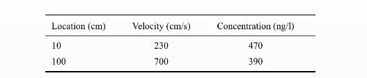
An indirect way of measuring of secondary emission from ponds or large bodies of water used in waste treatment is to measure the concentration and velocity over the surface. The data can then be fitted to a model of the type presented.In a typical experiment benzene concentration and velocity were
Chemical vapor deposition (CVD) on an inclined susceptor: a case-study problem. An important application of convective mass transfer theory is in CVD processes employed to coat surfaces with thin films of metals or semi-conductors. In fact, this turns out to be an example of simultaneous heat and
Mass transfer from a bubble. Calculate the mass transfer coefficient for the air-water system for bubbles rising at a gas velocity of \(5 \mathrm{~cm} / \mathrm{s}\) in a pool of stagnant liquid. Use the penetration model for \(k_{\mathrm{L}}\).
Axial dispersion in channel flow. Consider the pressure-driven laminar flow in a channel of height \(2 h\). Derive the following formula for the axial dispersion coefficient:\[D_{\mathrm{E}}=\frac{2 h^{2}\langle vangle^{2}}{105 D}\]Here \(\langle vangle\) is the averaged velocity and \(D\) is the
Axial dispersion in turbulent flow. Taylor showed that the following expression is suitable for the calculation of the axial dispersion coefficient for turbulent flow in a pipe:\[D_{\mathrm{E}}=10 R V_{\mathrm{f}}\]Here \(R\) is the pipe radius and \(V_{\mathrm{f}}\) is the friction velocity. Show
A model for a hemodialyser with simulation of the patient-artificial-kidney system: a case-study problem. A useful case study is the paper by Ramachandran and Mashelkar (1980), where a mesoscopic model with axial dispersion was used for the blood side and plug flow was used for the dialysate side.
A model for chromatographic separation: a case-study problem. An important application of Taylor dispersion is in chromatography. Here pulses of a mixture of solutes are introduced into one end of a packed-bed reactor containing an adsorbent and washed through the bed with a solvent. Since
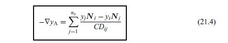
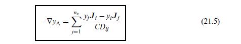
Show that the two representations of the Stefan-Maxwell model given by Eqs. (21.4) and (21.5) are equivalent. ns -VA = j=1 y;Ni-yiNj CDij (21.4)
Show that the Stefan-Maxwell model can be rearranged to define a pseudo-binary diffusivity, \(D_{i \mathrm{~m}}\), for species \(i\) in the mixture:\[\frac{1}{D_{i \mathrm{~m}}}=\frac{\sum_{k=1}^{N}\left(y_{k}-y_{j} N_{k} / N_{j}\right) / D_{j k}}{1-y_{j} \sum_{k}\left[N_{k} / N_{j}\right]}\]The
Support for the form of the generalized version of Fick's law introduced in this chapter can be found in the thermodynamics of irreversible processes. Here we introduce a brief description of this field. More detailed descriptions can be found in the books by Hase (1968) and De Groot and Mazur
Acetone is evaporating in a mixture of nitrogen and helium. Find the rate of evaporation and compare it with the rates in pure nitrogen and pure helium. Also compare it with the model using a pseudo-binary diffusivity value for acetone. The pseudo-binary diffusivity can be calculated from the
Catalytic oxidation of \(\mathrm{CO}\) is an important reaction in pollution prevention. The reaction scheme is\[\mathrm{O}_{2}(\mathrm{~A})+2 \mathrm{CO}(\mathrm{B}) \rightarrow 2 \mathrm{CO}_{2}(\mathrm{C})\]Set up the Stefan-Maxwell model for this problem. State the determinacy condition and
Examine how the rank of the stoichiometric matrix can be used to reduce the number of equations to be solved. For example, if there are \(n_{\mathrm{s}}\) components and \(n_{\mathrm{r}}\) equations we can show that only \(n_{\mathrm{s}}-n_{\mathrm{r}}\) independent mass-balance equations are
Extend the analysis two reactions, making it applicable for steam reforming of methane. The first reaction is\[\mathrm{CH}_{4}+\mathrm{H}_{2} \mathrm{O} \rightleftharpoons \mathrm{CO}+3 \mathrm{H}_{2}\]and this is followed by the water-gas shift reaction shown in the text. Kinetic and diffusion
Consider the three-component system consisting of acetaldehyde (1), hydrogen (2), and ethanol (3). The binary diffusivity values at \(548 \mathrm{~K}\) and \(101.3 \mathrm{kPa}\) are given in Example 21.3.Find the \(K\) matrix at the bulk gas composition and at the catalyst surface concentration.
In the matrix representation the species \(n\) chosen for elimination is usually referred to as the solvent. The choice of "solvent" species is arbitrary, but it can have an effect on the coefficient and the structure of the resulting form as shown below.A system with a very large variation in
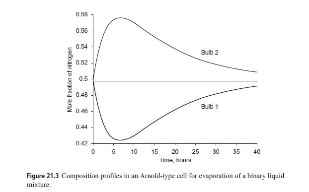
Derive the solutions for transient concentration profiles in the two-bulb apparatus (Example 21.5 in the text) for the binary case, and show that the multicomponent case can be derived as an extension of this. What assumption is implicit in extending the binary case to the multicomponent
When two gases A and B are forced to diffuse through a third gas C, there is a tendency of A and \(\mathrm{B}\) to separate because of the difference in their diffusivities in gas \(\mathrm{C}\). This phenomenon could possibly be used for isotope separation. Consider a "diffusion tube" of diameter
Show that another way of writing the flux due to pressure diffusion is in terms of partial molar volume and the total mixture density is\[J_{\mathrm{A}}^{*}(\text { pressure diffusion })=-C D_{\mathrm{AB}} \frac{1}{R_{\mathrm{G}} T}\left(\tilde{V}_{\mathrm{A}}-\tilde{V}\right) abla P\]
Estimate the steady-state concentration profile when a typical albumin solution is subjected to a centrifugal field of 30000 times the force of gravity under the following conditions: the cell length is \(1.0 \mathrm{~cm}\), the molecular weight of albumin is 45000 , the apparent density of albumin
A mixture of \(\mathrm{H}_{2}\) and \(\mathrm{D}_{2}\) is contained in two bulbs connected by a porous plug. The bulbs are maintained at different temperatures of 200 and \(600 \mathrm{~K}\). The thermal diffusion parameter \(k_{T}=0.0166\). The mole fraction of deuterium is initially equal to 0.1
Verify that both the pressure and the vorticity field satisfy the Laplace equation for Stokes flow.Verify that the velocity field satisfies the biharmonic equation\[\begin{equation*}abla^{4} \boldsymbol{v}=0 \tag{15.81}\end{equation*}\]
Show that the force acting on a control surface of any arbitrary control volume is equal to the force on a larger regularly shaped control volume enclosing the given body. In order to do this you need a control volume that is multiply connected by surfaces \(S_{1}\) and \(S_{2}\). Then apply the
Confirm that the definition of the streamfunction given in the text satisfies the continuity equation.Use this in the N-S equation and derive the form for the \(E^{4}\) operator in spherical coordinates with \(\phi\) symmetry.
Consider the flow in cylindrical coordinates with no dependence on \(\theta\). How is the streamfunction defined? What is the non-vanishing component of vorticity. Show that the \(E^{2}\) operator takes the form\[\begin{equation*}E^{2}=\frac{\partial^{2}}{\partial r^{2}}-\frac{1}{r}
Derive the general solution for \(\psi\) given in the text (Eq. (15.9)). 0 (r,n) = A++ Bnr "+1 + Cnr -" + Dnr"1Qn(n) 2-n (15.9) n=1
What are units for \(C_{1}\) in Eq. (15.10)? Confirm that the units agree on both sides. F = 4 (15.10)
A sphere of radius \(R\) is rotating in an infinite fluid at an angular velocity of \(\Omega\). Derive the following expression for the velocity field:\[v_{\phi}=r \Omega \sin \theta \frac{R^{3}}{r^{3}}\]Find an expression for the torque exerted by the sphere on the fluid. Assume a solution of the
Find the solution to Stokes flow past a sphere where the far-field velocity satisfies the elongational flow defined as \(v_{x}=\dot{\gamma} x, v_{y}=\) \(\dot{\gamma} y\), and \(v_{z}=-2 \dot{\gamma} z\).First verify that the continuity equation is satisfied. Then transform the velocity to
The general solution to Stokes flow in 2D Cartesian coordinates. For the 2D case the governing equation is \(abla^{4} \psi=0\). The operator \(abla\) may be applied either in Cartesian \((x, y)\) or in polar \((r, \theta)\) coordinates. In either case it would be appropriate to seek a general form
The case of flow past a cylinder of infinite length normal to the axis was also studied by Stokes. In view of the 2D nature of the problem, it is more convenient to work in \(r, \theta\) coordinates. The governing equation is \(abla^{4} \psi=0\).What are the boundary conditions that can be imposed
Verify the vector identity\[\begin{equation*}abla^{2} \boldsymbol{v}=abla(abla \cdot \boldsymbol{v})-abla \times(abla \times \boldsymbol{v}) \tag{15.83}\end{equation*}\]
Show that, for irrotational axisymmetric flows in cylindrical coordinates, the streamfunction satisfies the following equation:\[\frac{\partial^{2} \psi}{\partial r^{2}}-\frac{1}{r} \frac{\partial^{2} \psi}{\partial \theta^{2}}+\frac{\partial^{2} \psi}{\partial z^{2}}=0\]
Indicate the type of flow given by \(\phi=\sqrt{r} \cos (\theta / 2)\). Calculate and plot typical streamlines.
Consider a source of flow in \(3 \mathrm{D}\) of strength \(S\) (dimensions \(L^{3} / T\) ), Then the flow is axisymmetric and independent of the \(\theta\)-direction in the spherical coordinate system. Show by a mass balance that\[S=4 \pi r^{2} v_{r}\]and hence derive Eq. (15.41) for the potential
Verify the principle of superposition, which states that if \(\phi_{1}\) and \(\phi_{2}\) are solutions to potential flow then \(\phi=c_{1} \phi_{1}+c_{2} \phi_{2}\) is also a solution.Also show that \(\phi_{1} \phi_{2}\) is NOT a solution.
Verify by direct substitution that the functions \(r^{n} \cos (n \theta)\) etc. shown in the text satisfy the Laplace equation in polar coordinates.Calculate the streamfunction for the above-mentioned potential function and construct a contour-plot of streamlines for \(n=1 / 2,1\), and 3/2. MATLAB
State the form of the Laplace equation in axisymmetric spherical coordinates.Verify that the following functions satisfy this equation:\[r \cos \theta ; \quad \cos \theta / r^{2}\]A linear combination is also a solution by superposition. Thus the following solution for \(\phi\) obtained by taking
A cylinder of diameter \(1.2 \mathrm{~m}\) and length \(7.5 \mathrm{~m}\) rotates at \(90 \mathrm{r}\).p.m. with its axis perpendicular to an air stream with an approach velocity of \(3.6 \mathrm{~m} / \mathrm{s}\).Plot the tangential component of the velocity along the circumference of the
Model equations similar to those for potential flow arise in flow in porous media, which has a wide variety of applications, e.g., in groundwater treatment, water-purity remediation, filtration, flow of a drug into a tissue such as a tumor, etc. The mathematical structure of the problem is
One way of cleaning up environmentally polluted underground water is to pump it out of the ground, treat it with some equipment (by catalytic or photochemical oxidation, for example), and then pump it back into the ground. This is referred to as the pump-and-treat process in the EPA jargon.Here we
Consider the flow past a flat plate. Here we examine the effect of a superimposed velocity \(v_{y 0}\) at the plate surface. This can be done by the integral method with only minor changes in the equations. Verify that the velocity in the \(y\)-direction is now given by\[\begin{equation*}v_{y
Find the value of \(m\) for which the wall shear stress is independent of the principal flow direction.Find the value of \(m\) for which the boundary-layer thickness is a constant.
Consider the problem of a semi-infinite fluid subject to a constant shear at the interface. This can be caused, for instance, by a surface-tension gradient. Show that the following differential equation is applicable for the boundary layer:\[3 f^{\prime \prime \prime}+2 f f^{\prime
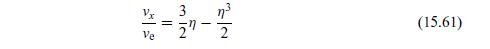
Von Kármán assumed a cubic profile for the integral momentum analysis over a flat plate. Since a cubic has four constants, four conditions were used.(i) \(V_{x}=0\) at \(y=0\).(ii) \(V_{x}=V_{\mathrm{e}}\) at \(y=\delta\).(iii) \(d V_{x} / d y=0\) at \(y=\delta\).(iv) \(d^{2} V_{x} / d y^{2}=0\)
Consider a boundary layer with no external pressure gradient (a flat plate). Then, from the Prandtl boundary-layer equation, deduce that\[\mu \frac{d^{2} v_{x}}{d y^{2}}=0 \text { at } y=0\]Now derive an expression for the second derivative of velocity at the surface for the case where there is a
A cubic approximation is commonly used in conjunction with the von Kármán momentum integral. An alternative form is the sine function:\[v_{x}=\alpha \sin (b y)\]What should the constants \(\alpha\) and \(b\) be in order to satisfy some conditions on \(v_{x}\) for a flatplate geometry? Repeat the
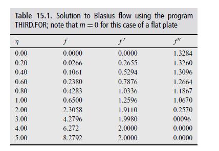
Follow up the derivations leading to the Blasius equation leading to\[f^{\prime \prime \prime}+f f^{\prime \prime}=0\]A useful routine to solve this is BVP4C in MATLAB. Solve the Blasius equation using this routine, and compare your answer with the results in Table 15.1. In particular, use the
The following system of differential equations arises in the modeling of a stirred tank reactor with an autocatalyic reaction:\[\begin{aligned}& \frac{d x}{d t}=x-x y \\& \frac{d y}{d t}=-y+x y+y^{2}\end{aligned}\]Find the steady states by setting the LHS to zero and solving the set of resulting
The Lorenz equation is widely used in the theory of non-linear equations and was encountered in modeling of natural convection. While working with these equations Lorenz discovered the phenomena of chaos. The system is described by the following set of differential equations:\[\begin{aligned}&
Analyze the Frank-Kamenetskii problem for the three standard geometries of slab, cylinder, and sphere. You will need to discretize the operators suitably for the cylinder and sphere. Plot the bifurcation diagram as a function of the thermicity parameter.
Verify the integral obtained by Rayleigh and hence show that the velocity profile needs to have an inflexion point for instability. Show that a simple shear flow is stable. Hence viscosity is needed to cause flow instability for such cases.
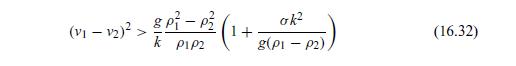
Derive the kinematic and dynamic conditions needed in the analysis. Set up the equations to find the constants. Now require that the determinant of the coefficient matrix should be zero to obtain a non-trivial solution. Hence verify the algebra leading to Eq. (16.32). 8 P-P (VI-V2) PIP2 (1 k ok
A shear layer between two fluids. Assume the following velocity distribution between two shear layers:\[v_{x}(y)=v_{0} \tanh (y / \delta)\]This is known as the Betchov and Criminale form. Calculate the stability analysis using the Rayleigh equation for the following parameters: \(v_{0}=1\) and
Stability of flow in torsional flow. Taylor determined the critical speed of rotation for flow between concentric cylinders with the inner cylinder rotating. The transition is characterized by a critical Taylor number, \(T a\), defined as\[T a=\frac{R_{\mathrm{o}}^{4}
Would the critical Rayleigh number for flow transition for the Bénard problem increase or decrease with the Prandtl number? Explain why in terms of the physics of the problem.
Stability analysis with heat transfer. Set up the equations for steady state for the Bénard problem.Now perturb the temperature and use an energy equation to derive an equation for the temperature perturbation. This in turn needs an equation for the velocity profile. Derive this equation.Thus we
Chandrasekhar (1961) has shown that the above (Bénard) problem can be solved in terms of the vorticity, which reduces the problem to a sixth-order eigenvalue problem for the perturbation in temperature. Your task is to work through the algebra and set up this sixth-order problem. Then you can try
Search the literature or web and discuss briefly the principles behind the following flowmeasurement devices: a Pitot tube; a hot-wire anemometer; a laser-Doppler velocity meter; and a radioactive-particle tracker. Also comment on the utility of these devices in the study of turbulent flow.
Explain the significance of the following cross-correlation terms:\[\begin{aligned}& \overline{v_{x}^{\prime} v_{y}^{\prime}} \\& \overline{v_{x}^{\prime} T^{\prime}} \\& \overline{v_{x}^{\prime} C_{\mathrm{A}}^{\prime}} \\&\overline{C_{\mathrm{A}}^{\prime} C_{\mathrm{A}}^{\prime}} \\&
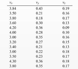
The following data were obtained for the velocity profiles in turbulent flow at a specified point in a channel flow as a function of time. The measurements were taken 0.01 seconds apart. The velocity was reported in \(\mathrm{m} / \mathrm{s}\).Find the mean velocity, the turbulent stress tensor
Verify that the fluctuating component of velocity (2D assumption) satisfies the following equation:\[\begin{equation*}\frac{\partial v_{x}^{\prime}}{\partial x}+\frac{\partial v_{y}^{\prime}}{\partial y}=0 \tag{17.52}\end{equation*}\]The velocity components can be expanded as a Taylor series in
The velocity profile for turbulent flow in circular pipes is often approximated by the \(1 / 7\) thpower law:\[\bar{v}_{z}=v_{\max }(1-r / R)^{1 / 7}\]Find an expression for the cross-sectionally averaged velocity.A more general expression for the velocity profile is\[\bar{v}_{z}=v_{\max }(1-r /
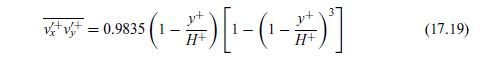
Use the equation (17.19) suggested by Pai for the turbulent stress and integrate for the velocity profile. How do the results compare with that of Prandtl? = 0.9835 H+ (1-#)['-(1-#)'] (17.19) H+
Water is flowing through a long pipe of diameter \(15 \mathrm{~cm}\) at \(300 \mathrm{~K}\). The pressure gradient is \(500 \mathrm{~Pa} / \mathrm{m}\).Using the Blasius equation for the friction factor find the volumetric flow rate and the average velocity. Then find the maximum velocity and the
Water is flowing in a pipe of diameter \(20 \mathrm{~cm}\) with a pressure gradient of \(3000 \mathrm{~Pa} / \mathrm{m} . \mu=\) \(0.001 \mathrm{~Pa} \cdot \mathrm{s}\).Find the wall shear stress.Find the friction velocity.Find the thickness of the laminar sublayer.Find the velocity at
Consider a fully developed flow of water in a smooth pipe of diameter \(15 \mathrm{~cm}\) at a flow rate of \(0.006 \mathrm{~m}^{3} / \mathrm{s}\).The pressure drop can be calculated by the Blasius relation for this case.Verify by an overall force balance that the wall shear stress is equal to \((R
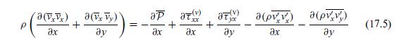
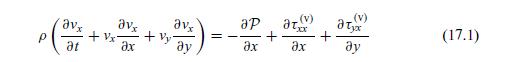
If the RANS equation (17.5) is subtracted from the unaveraged \(\mathrm{N}-\mathrm{S}\) equation (17.1), we obtain the following equation for the perturbation velocity:\[\begin{equation*}\frac{\partial v_{i}^{\prime}}{\partial t}+V_{j}\left(v_{i}^{\prime}, j\right)+v_{j}^{\prime}\left(V_{i},
Take the product of the perturbation velocity equation given by Eq. (17.53) by any component of the perturbation velocity. This results in an equation for \(v_{x}^{\prime} v_{y}^{\prime}\), which is the turbulent stress. Derive this equation and show that the triple correlation terms remain in this
Show that, for the isotropic case, (i) the velocity correlation function is now symmetric and (ii) the pressure-velocity correlation is zero.
Extend the analysis of the laminar-flow reactor for a power-law fluid. Perform some computations using the PDEPE solver, and show how the power-law index affects the conversion in the reactor.
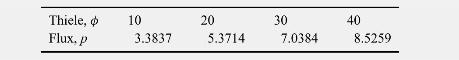
Perform the order-of \(-\epsilon^{2}\) approximation for the problem of diffusion with reaction in a catalyst of variable activity. Compare the flux with that obtained from the BVP4C solver in MATLAB. Perform computations for \(\phi\) of 10 , 20, and 30.The results are 9.7313. 19.7416, and 29.745,
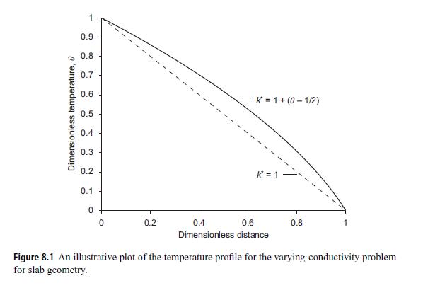
Express the Henry's-law constants reported in Table 8.1 as \(H_{i, p c}\) and \(H_{i, c p}\). Dimensionless temperature, 0.9 0.8 0.7 0.6 K=1+ (0-1/2) 0.5 0.4 0.3 0.2 0.1 K = 1 0 0.2 0.4 0.6 0.8 Dimensionless distance Figure 8.1 An illustrative plot of the temperature profile for the
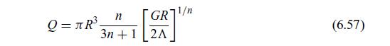
It is common to rearrange Eq. (6.57) to a friction-factor and Reynolds-number form similar to that for a Newtonian fluid. The friction factor is defined as usual by Eq. (1.22):\[f=\frac{1}{4} \frac{p_{0}-p_{l}}{ho\langle vangle^{2} / 2} \frac{d}{L}\]If one wishes to express the results by the same
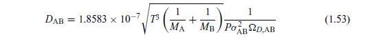
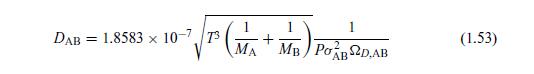
Find the binary pair diffusivity for the system methane (A)-ethane (B) at \(293 \mathrm{~K}\) and \(1 \mathrm{~atm}\) by using the Lennard-Jones method given by Eq. (1.53) by the following methods.(a) Use the following parameters (from the BSL book): \(\sigma_{\mathrm{A}}=3.780 Å\) and
Consider expansion of a function in terms of a series \(F_{n}(x)\) in the following form:\[f(x)=\sum_{n} A_{n} F_{n}(x)\]If the functions \(F_{n}\) are orthogonal then this property helps to unfold the series and permits us to find the series coefficients, one at a time.State what is meant by
The fact that the eigenfunctions are orthogonal can be verified easily using the symbolic calculations in MATLAB or MAPLE. But the underlying theory is based on the SturmLiouville problem. You may wish to explore this further by looking at some books.State what a Sturm-Liouville equation is.Prove
There is nothing magical about the eigenfunctions being orthogonal. This can be shown by integration by parts twice.Consider two eigenfunctions \(F_{n}\) and \(F_{m}\), both of which satisfy the following equations:\[\begin{equation*}\frac{d^{2} F_{n}}{d x^{2}}=-\lambda_{n}^{2} F_{n}
Analyze the transient problem with the Dirichlet condition for a long cylinder and for a sphere. Derive expressions for the eigenfunctions, eigenconditions, and eigenvalues. Find the series coefficients for a constant initial temperature profile.
A concrete wall \(20 \mathrm{~cm}\) thick is initially at a temperature of \(20^{\circ} \mathrm{C}\), and is exposed to steam at pressure \(1 \mathrm{~atm}\) on both sides. Find the time for the system to reach a nearly steady state. Find the rates of condensation of steam at various values of
A finite cylinder is \(2 \mathrm{~cm}\) in diameter and \(3 \mathrm{~cm}\) long and at a temperature of \(200^{\circ} \mathrm{C}\), and is cooled in air at \(30^{\circ} \mathrm{C}\). The convective heat transfer coefficient is estimated as \(10 \mathrm{~W} / \mathrm{m}^{2} \cdot \mathrm{K}\).
For the Biot problem in a slab by expanding the sin and cos term and keeping only terms up to \(\lambda^{2}\) the following approximate relation can be obtained for the eigenvalues for small Biot number:\[\lambda=\sqrt{B i /(1+B i / 2)}\]Verify the result.Find the value for a Biot number of 1 , and
Consider the problem of transient heat transfer with a constant heat source in a slab.Show that the governing equation in dimensionless form is\[\begin{equation*}\frac{\partial \theta}{\partial t^{*}}=\frac{\partial^{2} \theta}{\partial \xi^{2}}+1 \tag{11.83}\end{equation*}\]Identify and define the
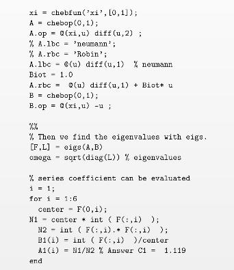
Eigenvalues without pain: CHEBFUN code. Eigenfunctions can be derived using the CHEBFUN with MATLAB since it has an overloaded eig function. The following code solves for the eigenfunctions of the Robin. The code can also readily evaluate the series coefficient. Thus the whole procedure of the
A hot dog at \(5^{\circ} \mathrm{C}\) is to be cooked by dipping it in boiling water at \(100^{\circ} \mathrm{C}\). Model the hot dog as a long cylinder with a diameter of \(20 \mathrm{~mm}\). Find the cooking time, which is defined as the time, for the center temperature to reach \(80^{\circ}
Assume that the asympotic solution has a time-dependent part, which is linear in time, and a positiondependent solution, which is an unknown function. Thus the solution should be of the following form:\[\theta_{\text {asy }}=A \tau+F(\xi)\]where \(A\) is a constant to be determined. The linear
A slab has a thermal diffusivity of \(5 \times 10^{-6} \mathrm{~m}^{2} / \mathrm{s}\) and is fairly thick. The initial temperature is \(300 \mathrm{~K}\) and the surface temperature is raised to \(600 \mathrm{~K}\) at time zero. Find the temperature \(0.5 \mathrm{~m}\) below the surface after one
Consider the problem of transient diffusion in a composite slab with two different thermal conductivities. Thus region 1 extending from 0 to \(\kappa\) has a thermal conductivity \(k_{1}\), while the region 2 from \(\kappa\) to 1 has a conductivity of \(\kappa_{2}\). The slab is initially at a
A large tank filled with oxygen has an initial concentration of oxygen of \(2 \mathrm{~mol} / \mathrm{m}^{3}\). The surface concentration on the liquid side of the interface is changed to \(9 \mathrm{~mol} / \mathrm{m}^{3}\) and maintained at this value.Calculate and plot the concentration profile
Consider the drug-release problem in the text, but now the drug is in the form of a cube with sides \(0.652 \mathrm{~cm}\). Find the center concentration after \(48 \mathrm{~h}\) and the fraction of drug released.
A porous cylinder, \(2.5 \mathrm{~cm}\) in diameter and \(80 \mathrm{~cm}\) long, is saturated with alcohol and maintained in a stirred tank. The alcohol concentration at the surface of the cylinder is maintained at \(1 \%\). The concentration at the center is measured by careful sampling and is

Showing 1000 - 1100 of 1819

First
4
5
6
7
8
9
10
11
12
13
14
15
16
17
18
Last

Step by Step Answers

Services

Sitemap
Fun
Definitions
Become Tutor
Used Textbooks
Study Help Categories
Recent Questions
Expert Questions
Campus Wear
Sell Your Books

Company Info

Security
Copyrights
Privacy Policy
Terms & Conditions
SolutionInn Fee
Scholarship
Online Quiz
Give Feedback, Get Rewards

Get In Touch

About Us
Contact Us
Career
Jobs
FAQ
Student Discount
Campus Ambassador

Secure Payment

Download Our App

© 2026 SolutionInn. All Rights Reserved