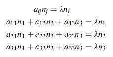
New Semester Started Get 50% OFF Study Help! --h --m --s Claim Now

Question Answers

Textbooks

Find textbooks, questions and answers

Oops, something went wrong!

Change your search query and then try again

Result Not Found

Books FREE
Study Help
Tutors
AI Study Planner NEW
Sell Books

Search
Sign In
Register

study help
engineering
elasticity theory applications

Elasticity Theory Applications And Numerics 4th Edition Martin H. Sadd Ph.D. - Solutions

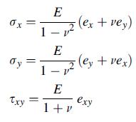
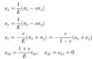
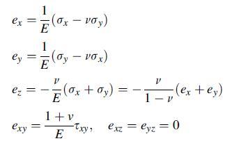
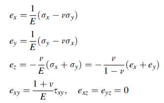
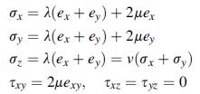
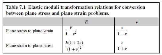
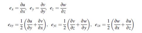
Invert the plane stress form of Hooke’s law (7.2.2) and express the stresses in terms of the strain components:Equation 7.2 .2 0x = dy Txy E -(ex + vey) 1- E 1- E 1+v -(ey + vex) exy
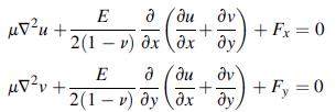
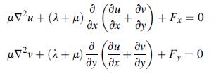
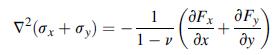
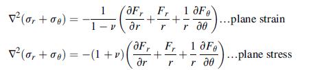
Using the results from Exercise 7.6 , eliminate the stresses from the plane stress equilibrium equations and develop Navier equations (7.2.5). Also, formally establish the Beltramie-Michell equation (7.2.7).Data from exercise 7.6 Invert the plane stress form of Hooke’s law (7.2.2) and express
For plane stress, investigate the unwanted three-dimensional results coming from integration of the strain-displacement relations involving the out-of-plane strains ez, exz, and eyz.
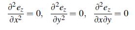
For the plane stress problem, show that the neglected nonzero compatibility relations involving the out-of-plane component ez are:Next integrate these relations to show that the most general form for this component is given by:where a, b, and c are arbitrary constants. In light of relation
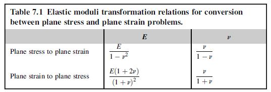
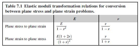
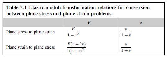
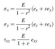
Using the transformation results shown in Table 7.1 , determine the required corresponding changes in Lame´’s constant λ and the shear modulus μ.Table 7.1 Table 7.1 Elastic moduli transformation relations for conversion between plane stress and plane strain problems. E Plane stress to plane
Verify the validity of the transformation relations given in Table 7.1 by:(a) Transforming the plane strain equations (7.1.5) and (7.1.7) into the corresponding plane stress results.(b) Transforming the plane stress equations (7.2.5) and (7.2.7) into the corresponding plane strain
Verify the validity of the transformation relations given in Table 7.1 by:(a) Transforming the plane strain Hooke’s law (7.1.3) into the corresponding plane stress results given in Exercise 7.6 .(b) Transforming the plane stress Hooke’s law (7.2.2) into the corresponding plane strain results
7.13 For the pure bending problem shown in Example 8.2 , the plane stress displacement field was determined and given by relations (8.1.22)2 as:Equation 8.1 .22Using the appropriate transformation relations from Table7.1 , determine the corresponding displacements for the plane strain case. Next
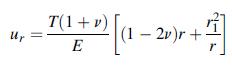
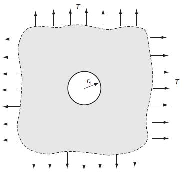
Consider the problem of a stress-free hole in an infinite domain under equal and uniform farfield loading T, as shown in Fig. 8.11 . The plane strain radial displacement solution for this problem is found to be:where r1 is the hole radius. Using the appropriate transformation relations from
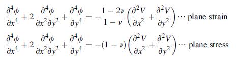
Explicitly develop the governing equations (7.5.4) in terms of the Airy function for plane strain and plane stress.Equation 7.5 .4 ap dx4 ap 24 + axa ay4 +2. ap ato + axay ay atd +2. 0x4 1-2v (8v 0 v + 22). 1-va dy av av - (1 - v)| + a ay plane strain plane stress
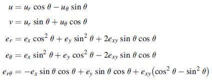
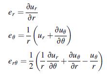
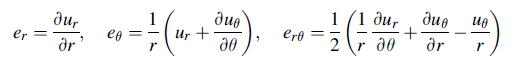
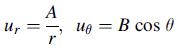
Derive the polar coordinate strain-displacement relations (7.6.1) by using the transformation equations:Equation 7.6 .1 u= ur cos 0 - ue sin 0 v=u, sin + ug cos 0 er ex cos 0 + ey sin 0 +2exy sin 0 cos 0 eg = ex sin 0 + ey cos 0 - 2exy sin 0 cos 0 ere = ex sin0 cos + ey sin cos + exy (cos 0-sin0)
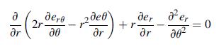
Using the polar strain-displacement relations (7.6.1), derive the strain-compatibility relation:Equation 7.6 .1 (2 2r 20 2 r +rar 202 aer = 0
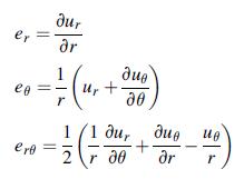
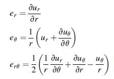
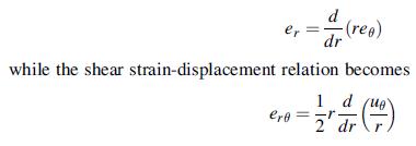
For the axisymmetric polar case where all field functions depend only on the radial coordinate r, show that a strain compatibility statement can expressed as: er = d ere - (rea) dr while the shear strain-displacement relation becomes 1 due dr (H)
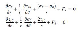
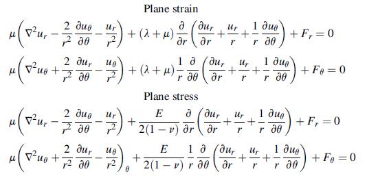
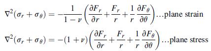
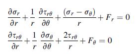
For the plane strain case, starting with the equilibrium equations (7.6.3), develop Navier equations (7.6.4)1,2. Also verify the compatibility relation (7.6.6)1.Equation 7.6 .3Equation 7.6 .4Equation 7.6 .6 1 r tre (ar - ae) + r 20 r tre ar + 1 + 2 r + + Fr = 0 Fo= 0
For the plane stress case, starting with the equilibrium equations (7.6.3), develop Navier equations (7.6.4)3,4. Also verify the compatibility relation (7.6.6)2.Equation 7.6 .3Equation 7.6 .4Equation 7.6 .6 ar 1 tre. (ar - ae) + - + ar tre, 1 20 + - r r 20 r + Fr = 0 + + Fo= 0
Using the chain rule and stress transformation theory, develop the stress–Airy function relations (7.6.7). Verify that this form satisfies equilibrium identically.Equation 7.6 .7 Or G0 tre 104 1024 + rr 30 2 ar2 r G 10 r de
For rigid-body motion, the strains will vanish. Under these conditions, integrate the strain–displacement relations (7.6.1) to show that the most general form of a rigid-body motion displacement field in polar coordinates is given by:Equation 7.6 .1where a, b, c are constants. Also show that
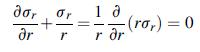
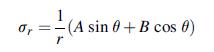
Consider the two-dimensional plane stress field of the form σr = σr(r, θ), σθ = τ rθ = 0. This is commonly referred to as a radial stress distribution. For this case, first show that the equilibrium equations reduce to:Next integrate this result to get σr = f(θ)/r where f(θ) is an
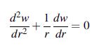
Consider the antiplane strain problem of a distributed loading F (per unit length) along the entire z-axis of an infinite medium. This will produce an axisymmetric deformation field.Using cylindrical coordinates, show that in the absence of body forces, governing equation (7.4.5) will reduce
Determine the strain and rotation tensors eij and ωij for the following displacement fields:a. b. c. where A, B, and C are arbitrary constants. u=Axy, v = Byz, w = C(x + z)
A two-dimensional displacement field is given by u = k(x2 + y2), v = k(2x–y), w = 0, where k is a constant. Determine and plot the deformed shape of a differential rectangular element originally located with its left bottom corner at the origin as shown. Finally, calculate the rotation component
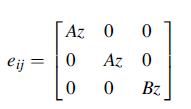
A three-dimensional elasticity problem of a uniform bar stretched under its own weight gives the following strain field:where A and B are constants. Integrate the strainedisplacement relations to determine the displacement components and identify all rigid-body motion terms. eij Az 0 0 Az 0 0 0 0 Bz
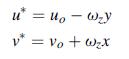
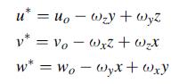
Explicitly verify that the general rigid-body motion displacement field given by (2.2.10) yields zero strains. Next, assuming that all strains vanish, formally integrate relations (2.2.5) to develop the general form (2.2.10).Equation 2.2.10Equation 2.2.5 u* = uo-wy + wyz v = vo - Wx + wX Vo w* = Wo
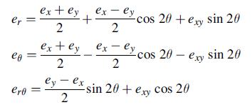
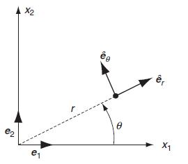
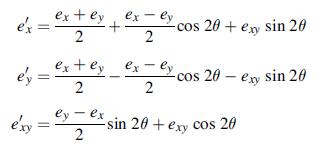
For polar coordinates defined by Fig. 1.8 , show that the transformation relations can be used to determine the normal and shear strain components er, eq, and erq in terms of the corresponding Cartesian components:Fig 1.8 er = ex+ey ex-ey, -+ 2 2 eo = ero = ex+ey 2 ey - ex 2 -cos 20 +exy sin 20
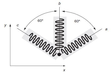
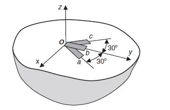
A rosette strain gage is an electromechanical device that can measure relative surface elongations in three directions. Bonding such a device to the surface of a structure allows determination of elongational strains in particular directions. A schematic of one such gage is shown in the following
A two-dimensional strain field is found to be given by ex =0.002, ey = –0.004, and exy = 0.001. Incorporating the transformation relations (2.3.6) into a MATLAB code, calculate and plot the new strain components in a rotated coordinate system as a function of the rotation angle θ. Determine the
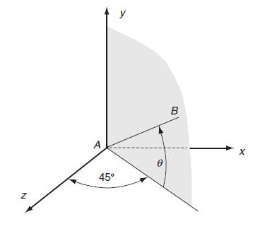
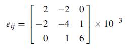
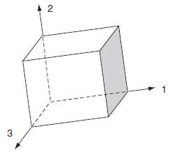
A three-dimensional strain field is specified by:Determine information on the strains in the shaded plane in the following figure that makes equal angles with the x- and z-axes as shown. UseMATLAB_ to calculate and plot the normal and inplane shear strain along line AB (in the plane) as a function
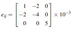
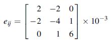
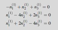
Using MATLAB, determine the principal values and directions of the following state of strain: eij 2-2 -2 0 -2 -4 1 0 16 10-3
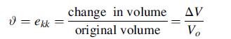
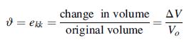
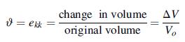
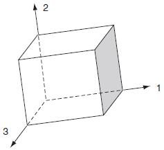
A rectangular parallelepiped with original volume Vo is oriented such that its edges are parallel to the principal directions of strain as shown in the following figure. For small strains, show that the dilatation is given by: d = ekk change in volume_AV original volume Vo
Determine the spherical and deviatoric strain tensors for the strain field given in Exercise 2.10. Justify that the first invariant or dilatation of the deviatoric strain tensor is zero. In light of the results from Exercise 2.11, what does the vanishing of the dilatation imply?Data from exercise
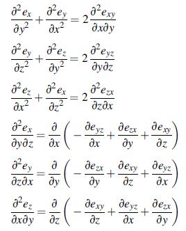
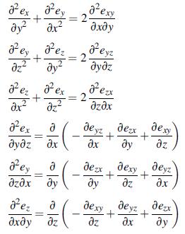
Using scalar methods, differentiate the individual strain displacement relations for ex, ey, and exy, and independently develop the first compatibility equation of set (2.6.2).Equation 2.6.2 Pex ey 2 ey de 2 + az2 + Fez Fex 0;2 dx 2ex z Fey z , z aexy = 2 Feyz z = 2. Fezx z + - - - + a
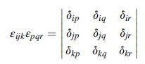
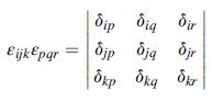
Using relation (1.3.5), show that the compatibility relations (2.6.1) with l = k can be expressed by nij = εiklεjmpelp,km = 0, which can also be written in vector notation as ∇ × e× ∇ = 0.Equation 1.3.5Equation 2.6.1 Eijk Epqr i ig Sir jp Sjg Sjr Skp Skg Skr
In light of Exercise 2.14 , the compatibility equations (2.6.2) can be expressed as nij = εikl εjmpelp,km = 0, where nij is sometimes referred to as the incompatibility tensor (Asaro and Lubarda, 2006). It is observed that hij is symmetric, but its components are not independent from one
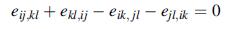
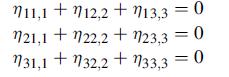
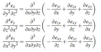
Show that the six compatibility equations (2.6.2) may also be represented by the three independent fourth-order equations:Equation 2.6.2 J ex ?z2 z 24ey azax 34e. 2 23 z 23 z z + z + + z + + z z x +
Determine if the following strains satisfy the compatibility equations (2.6.2):a. b. c. where A, B and C are constants.Equation 2.6.2 ex=Ay, ey = ez = 0, exy = (Ax+Bz)/2, eyz = Bxz + Cy, ezx = C.x
Show that the following strain field:gives continuous, single-valued displacements in a simply connected region only if the constants are related by A = 2B/3. ex = Ay, ey = Ax, exy = Bxy(x+y), ez = exz = Cyz =0
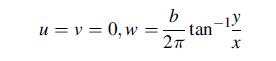
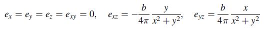
In order to model dislocations in elastic solids, multivalued displacement fields are necessary. As shown later in Chapter 15, for the particular case of a screw dislocation the displacements are given by:where b is a constant called the Burgers vector. Show that the strains resulting from these
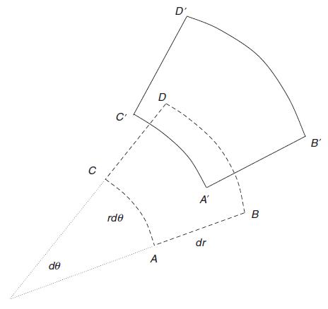
Consider the plane deformation of the differential element ABCD defined by polar coordinates r, θ as shown in the following figure. Using the geometric methods outlined in Section 2.2, investigate the changes in line lengths and angles associated with the deformation to a configuration
Using the results from Exercise 2.20, determine the two-dimensional strains er, eθ, erθ for the following displacement fields:a. b. c. where A, B, and C are arbitrary constants.Data from exercise 2.20Consider the plane deformation of the differential element ABCD defined by polar coordinates
Consider the cylindrical coordinate description for problems with axial symmetry such that all fields depend only on the radial coordinate r and the axial coordinate z. Determine the reduced strain displacement relations for this case. Further reduce these equations for the case with uθ = 0.
Consider the spherical coordinate description for problems with radial symmetry such that all fields depend only on the radial coordinate R. Determine the reduced strain displacement relations for this case. Further reduce these equations for the case with u∅ = uθ = 0.
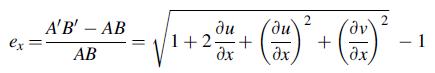
In Section 2.2 , before employing any small deformation assumptions, the two-dimensional extensional strain component ex was expressed as:We now wish to investigate the nature of small deformation theory by exploring this non-linear relation for the special case with linear displacement field
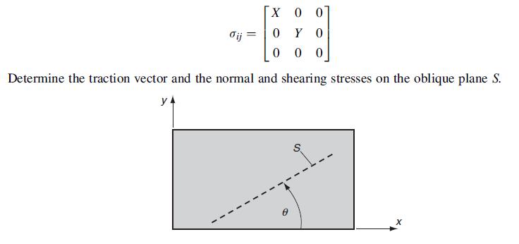
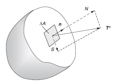
The illustrated rectangular plate is under uniform biaxial loading which yields the following state of stress: dij X 0 0 Y O 0 000 Determine the traction vector and the normal and shearing stresses on the oblique plane S. 4 X
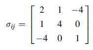
Using suitable units, the stress at a particular point in a solid is found to be:a. b. Determine the traction vector on a surface with unit normal (cos θ, sin θ, 0), where θ is a general angle in the range 0 ≤ θ ≤π . Plot the variation of the magnitude of the traction vector ΙTnΙ as a
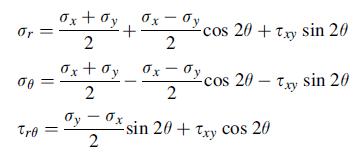
Show that the general two-dimensional stress transformation relations can be used to generate relations for the normal and shear stresses in a polar coordinate system in terms of Cartesian components: Or = = Tro = x + ay 2 + x + ay 2 2 0x - y 2 cos 20+ xy sin 20 exy cos 20-Txy sin 20 2 sin 20+ Txy
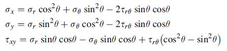
Verify that the two-dimensional transformation relations giving Cartesian stresses in terms of polar components are given by: ge sin0- 2tre sino coso cos0 - 2tre sino cost 0x = arcos0+ y = 0, sin0 + Txy = 0, sine cos0 - 0 sino cose + re (cos0 - sin0)
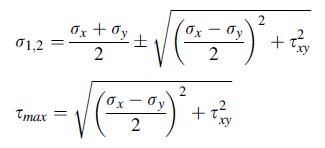
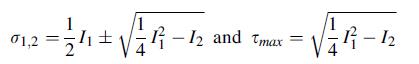
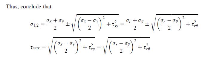
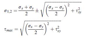
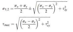
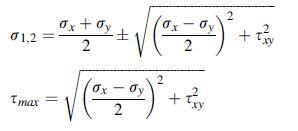
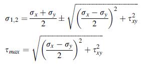
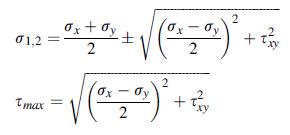
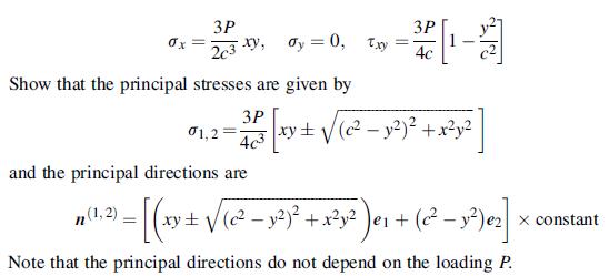
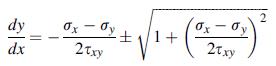
A two-dimensional state of plane stress in the x, y-plane is defined by σz = τ yz = τ zx = 0. Using general principal value theory, show that for this case the in-plane principal stresses and maximum shear stress are given by: 2 ax+ay ax - ay 72="+" = (727) + 3 01,2 Tmax= Ox-ay 2 2 + z
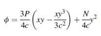
Explicitly verify relations (3.5.4) for the octahedral stress components. Also show that they can be expressed in terms of the general stress components by:Equation 3.5.4 Joct = 73 (0x + a + a) oy- - 3 - [(ox ay) + (ay a) + (a 0x) + 62y +6732 +67 ]/ - 1/2 Toct=
For the plane stress case in Exercise 3.5, demonstrate the invariant nature of the principal stresses and maximum shear stresses by showing that:Data from exercise 3.5A two-dimensional state of plane stress in the x, y-plane is defined by σz = τ yz = τ zx = 0. Using general principal value
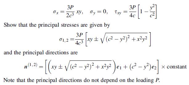
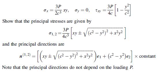
Exercise 8.2 provides the plane stress (see Exercise 3.5 ) solution for a cantilever beam of unit thickness, with depth 2c, and carrying an end load of P with stresses given by:Data from exercise 3.5A two-dimensional state of plane stress in the x, y-plane is defined by σz = τ yz = τ zx = 0.
Plot contours of the maximum principal stress σ1 in Exercise 3.8 in the region 0 ≤ x ≤ L, – c ≤ y≤ c, with L = 1, c = 0.1, and P = 1.Data from exercise 3.8Exercise 8.2 provides the plane stress (see Exercise 3.5) solution for a cantilever beam of unit thickness, with depth 2c, and
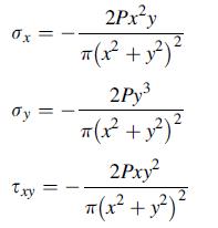
We wish to generalize the findings in Exercise 3.8 , and thus consider a stress field of the general form σij = Pfij (xk), where P is a loading parameter and the tensor function fij specifies only the field distribution. Show that the principal stresses will be a linear form in P, that is,
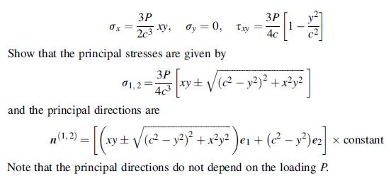
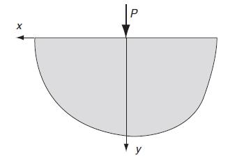
The plane stress solution for a semi-infinite elastic solid under a concentrated point loading is developed in Chapter 8. With respect to the axes shown in the following figure, the Cartesian stress components are found to be:Using results from Exercise 3.5, calculate the maximum shear stress at
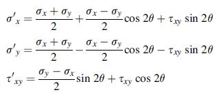
Show that shear stress S acting on a plane defined by the unit normal vector n (see Fig. 3.6) can be written as:Fig 3.6 S = [nn(01 02) + nnz (02 03) + nzn(03 01)]/
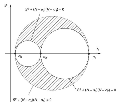
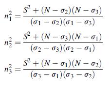
It was discussed in Section 3.4 that for the case of ranked principal stresses (σ1 > σ2 > σ3), the maximum shear stress was given by Smax = (σ1– σ3)/2, which was the radius of the largest Mohr circle shown in Fig. 3.7. For this case, show that the normal stress acting on the plane of maximum
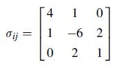
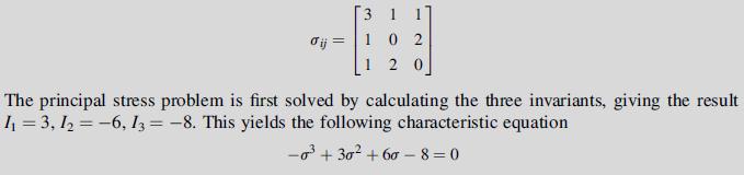
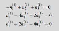
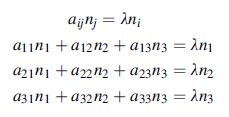
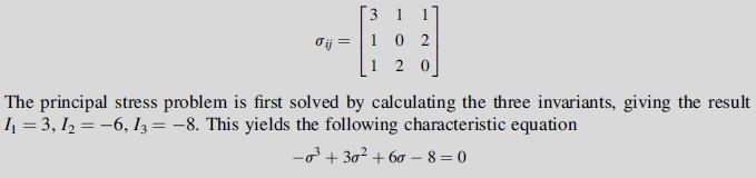
Explicitly show that the stress state given in Example 3.1 will reduce to the proper diagonal form under transformation to principal axes.Data from example 3.1For the following state of stress, determine the principal stresses and directions and find the traction vector on a plane with unit normal
Show that the principal directions of the deviatoric stress tensor coincide with the principal directions of the stress tensor. Also show that the principal values of the deviatoric stress σd can be expressed in terms of the principal values s of the total stress by the relation σd = σ–1/3
Determine the spherical and deviatoric stress tensors for the stress states given in Exercise 3.2.Data from exercise 3.2Using suitable units, the stress at a particular point in a solid is found to be. Determine the traction vector on a surface with unit normal (cos θ sin θ, 0), where θ is a
For the stress state given in Example 3.1, determine the von Mises and octahedral stresses defined in Section 3.5.Data from example 3.1For the following state of stress, determine the principal stresses and directions and find the traction vector on a plane with unit normal n = (0, 1, 1)/ √2:The
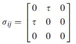
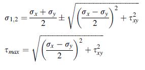
For the case of pure shear, the stress matrix is given by:where τ is a given constant. Determine the principal stresses and directions, and then using principal values compute the normal and shear stress on the octahedral plane. How could you determine N and S on the octahedral plane using the
For the two-dimensional plane stress case (see Exercise 3.5), show that the relationship between the maximum shear stress and von Mises stress is given by τ 2 max = 1/3 (σ2e—I21/4).Data from exercise 3.5A two-dimensional state of plane stress in the x, y-plane is defined by σz = τ yz =
For the stress state in Exercise 3.8, plot contours of the von Mises stress in the region 0≤x ≤L, –c≤ y≤ c, with L = 1, c = 0.1, and P = 1.Data from exercise 3.8Exercise 8.2 provides the plane stress (see Exercise 3.5) solution for a cantilever beam of unit thickness, with depth 2c, and
Starting with two-dimensional stress transformation relation (3.3.5), set dσ′x/dθ = 0, and thus show that the relation to determine the angle to the principal stress direction θp is given by tan 2θp = 2τ xy/σx–σy. Next explicitly develop relation (3.6.2).Equation 3.3.5Equation 3.6.2 o'x
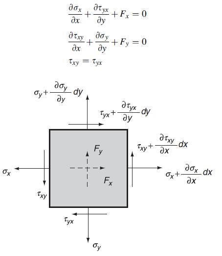
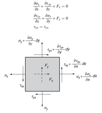
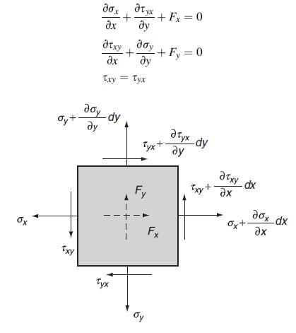
Consider the equilibrium of a two-dimensional differential element in Cartesian coordinates, as shown in the following figure. Explicitly sum the forces and moments and develop the two-dimensional equilibrium equations: Oyt Txy atyx ax + a txy + Txy = Tyx doy dy Tyx - + Fx = 0 Fy + +Fy = 0
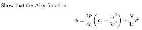
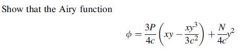
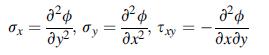
Consider the two-dimensional case described in Exercise 3.22 with no body forces. Show that equilibrium equations are identically satisfied if the stresses are expressed in the form:where ∅(x, y) is an arbitrary stress function. This stress representation will be used in Chapter 7 to establish a
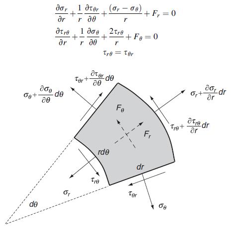
Following similar procedures as in Exercise 3.22 , sum the forces and moments on the two-dimensional differential element in polar coordinates (see figure), and explicitly develop the following two-dimensional equilibrium equations:Data from exercise 3.22Consider the equilibrium of a
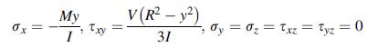
For a beam of circular cross-section, analysis from elementary strength of materials theory yields the following stresses:where R is the section radius, I = πR4/4, M is the bending moment, V is the shear force, and dM/dx = V. Assuming zero body forces, show that these stresses do not satisfy the
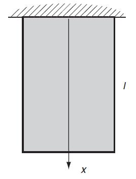
A one-dimensional problem of a prismatic bar (see the following figure) loaded under its own weight can be modeled by the stress field σx = σx(x), σy = σz = τ xy = τ yz = τ zx = 0, with body forces Fx = ρg, Fy = Fz = 0, where r is the mass density and g are the local acceleration of
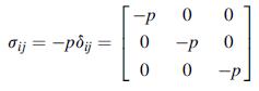
A hydrostatic stress field is specified by:where p = p (x1, x2, x3) and may be called the pressure. Show that the equilibrium equations imply that the pressure must satisfy the relation ∇p = F. aij =-poi ij 0 0 0 - - 0 - 0 0
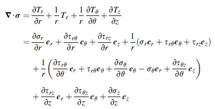
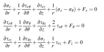
Verify the curvilinear cylindrical coordinate relations (3.8.5) and (3.8.6).Equation 3.8.5Equation 3.8.6 V.a , _ 1 + ar r , ar + er T, + + r 1tre 20 1. r 20 + dz -co + atr Zer + z airez+-(a,er + treeot Trez) z 20 er + Trole+ 20 at az ea+ az ; dz Zer -ager + +
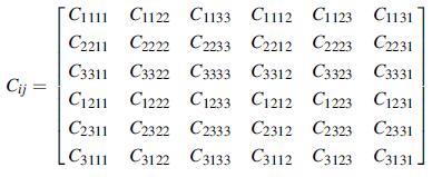
Show that the components of the Cij matrix in Eq. (4.2.2) are related to the components of Cijkl by the relation:Equation 4.2.2 Cij = C1 C1122 C1133 C1112 C1123 C1131 C2211 C2222 C2233 C2212 C2223 C2231 C3311 C3322 C3333 C3312 C3323 C3331 C1211 C1222 C1233 C1212 C1223 C1231 C2311 C2322 C2333 C2312
Explicitly justify the symmetry relations (4.2.4). Note that the first relation follows directly from the symmetry of the stress, while the second condition requires a simple expansion into the form ekl = 1/2 (ekl + elk) to arrive at the required conclusion.Equation 4.2.4 Cijkl = Cjikl Cijkl = Cijlk
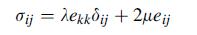
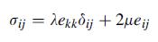
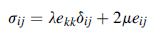
Substituting the general isotropic fourth-order form (4.2.6) into (4.2.3), explicitly develop the stress–strain relation (4.2.7).Equation 4.2.6Equation 4.2.3Equation 4.2.7 Cik = + ; + jk
For isotropic materials, show that the fourth-order elasticity tensor can be expressed in the following forms: Cijkl = ijkl + (ldjk + dik jl) Cjk = ( + ji) + (k u) ijki (oiljk Cijkl E -ijk! + 2(1 + v) Ev (1 + v) (1-2v) -(diljk + dikojl)
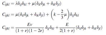
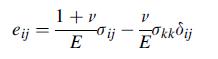
Following the steps outlined in the text, invert the form of Hooke’s law given by (4.2.7) and develop form (4.2.10). Explicitly show that E = μ(3λ + 2μ)/(λ + μ) and v = λ/[2(λ + μ)].Equation 4.2.7Equation 4.2.10 gij = kekkoij +2u ij
Using the results of Exercise 4.5, show that μ = E/ [2(1 + v)] and λ = Ev/ [(1 + v) (1 – 2v)].Data from exercise 4.5Following the steps outlined in the text, invert the form of Hooke’s law given by (4.2.7) and develop form (4.2.10). Explicitly show that E = μ(3λ + 2μ)/ (λ + μ) and v =
For isotropic materials show that the principal axes of strain coincide with the principal axes of stress. Further, show that the principal stresses can be expressed in terms of the principal strains as σi = 2μei + λekk.
A rosette strain gage (see Exercise 2.7) is mounted on the surface of a stress-free elastic solid at point O as shown in the following figure. The three gage readings give surface extensional strains ea = 300 × 10–6, eb = 400× 10–6, ec= 100×10–6. Assuming that the material is steel with
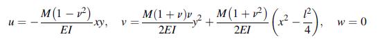
The displacements in an elastic material are given by:where M, E, I, and l are constant parameters. Determine the corresponding strain and stress fields and show that this problem represents the pure bending of a rectangular beam in the x,y plane. U M(1-1) EI -xy, M(1 + v)v 2EI V=- M(1 +1) (-2).
If the elastic constants E, k, and μ are required to be positive, show that Poisson’s ratio must satisfy the inequality –1 < v < 1/2. For most real materials it has been found that 0 < v < 1/2. Show that this more restrictive inequality in this problem implies that λ > 0.
Under the condition that E is positive and bounded, determine the elastic moduli λ, μ, and k for the special cases of Poisson’s ratio: v = 0, 1/4;1/2. Discuss the special circumstances for the case with v = 1/2.
Further explore the behaviors of the elastic moduli in Exercise 4.11 by making nondimensional plots of λ/E, μ/E and k/E for 0 ≤ v≤ 0.5.Data from exercise 4.11Under the condition that E is positive and bounded, determine the elastic moduliλ, μ, and k for the special cases of Poisson’s
Consider the case of incompressible elastic materials. For such materials, there will be a constraint on all deformations such that the change in volume must be zero, thus implying (see Exercise 2.11) that ekk = 0. First show that, under this constraint, Poisson’s ratio will become 12 and the
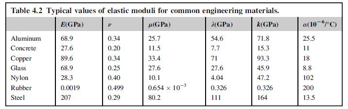
Consider the three deformation cases of simple tension, pure shear, and hydrostatic compression as discussed in Section 4.3 . Using the nominal values from Table 4.2 , calculate the resulting strains in each of these cases for:a. b. c. Note that for aluminum and steel, these tensile and shear
Show that Hooke’s law for an isotropic material may be expressed in terms of spherical and deviatoric tensors by the two relations: ij = 3kij, ij = 2ij
A sample is subjected to a test under plane stress conditions (specified by σz = τ zx = τ zy = 0) using a special loading frame that maintains an in-plane loading constraint σx = 2σy. Determine the slope of the stress strain response σx vs. ex for this sample.
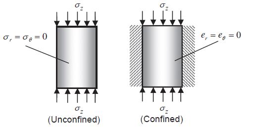
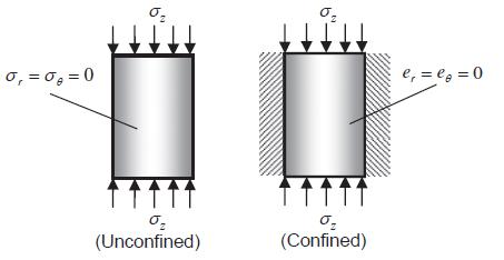
Using cylindrical coordinates, we wish to determine and compare the uniaxial stress strain response of both an unconfined and confined isotropic homogeneous elastic cylindrical sample as shown. For both cases we will assume that the shear stresses and strains will vanish. For the unconfined sample,
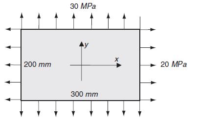
A rectangular steel plate (thickness 4 mm) is subjected to a uniform biaxial stress field as shown in the following figure. Assuming all fields are uniform, determine changes in the dimensions of the plate under this loading. 200 mm 30 MPa Ay 300 mm X 20 MPa
Redo Exercise 4.17 for the case where the vertical loading is 50 MPa in tension and the horizontal loading is 50 MPa in compression.Data from exercise 4.17Using cylindrical coordinates, we wish to determine and compare the uniaxial stress strain response of both an unconfined and confined isotropic
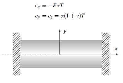
Consider the one-dimensional thermoelastic problem of a uniform bar constrained in the axial x direction but allowed to expand freely in the y and z directions, as shown in the following figure. Taking the reference temperature to be zero, show that the only nonzero stress and strain components are
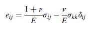
Verify that Hooke’s law for isotropic thermoelastic materials can be expressed in the form: 0x dy 0 Txy = E (1 + v) (1-2v) E (1 + v)(1-2v) -[(1 v)ex+v(ey + ez)] -[(1 = v)ey +v(ez + ex)] -[(1 = v)ez + v(ex + ey)] E (1 + v)(1-2v) E exy, 1+v Tyz = E -eyz, 1 + v Tzx = E 1 + v E 12v -a(T-To) E 1-2,
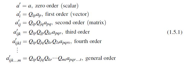
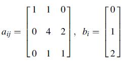
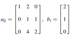
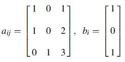
For the given matrix/vector pairs, compute the following quantities: aii, aijaij, aijajk, aijbj, aijbibj, bibj, bibi. For each case, point out whether the result is a scalar, vector or matrix. Note that aijbj is actually the matrix product [a]{b}, while aijajk is the product
Use the decomposition result (1.2.10) to express aij from Exercise 1.1 in terms of the sum of symmetric and antisymmetric matrices. Verify that a(ij) and a[ij] satisfy the conditions given in:the last paragraph.Equation 1.2.10Data from exercise 1.1For the given matrix/vector pairs, compute
If aij is symmetric and bij is antisymmetric, prove in general that the product aijbij is zero. Verify this result for the specific case by using the symmetric and antisymmetric terms from Exercise 1.2.Data from exercise 1.2Use the decomposition result (1.2.10) to express aij from Exercise 1.1 in
Explicitly verify the following properties of the Kronecker delta: djaj = a ai dijajk = aik
Formally expand the expression (1.3.4) for the determinant and justify that either index notation form yields a result that matches the traditional form for det[aij].Equation 1.3.4 det[ay]= |aj|= = all a12 a13 a21 922 a23 a31 a32 a33 = Eijka 1a2ja3k = = Eijka ilaj2 ak3
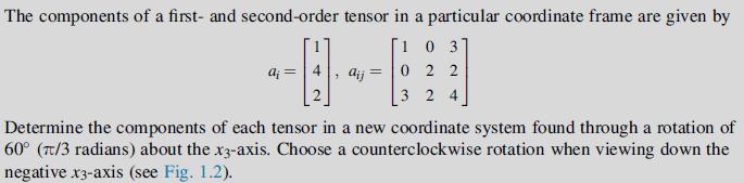
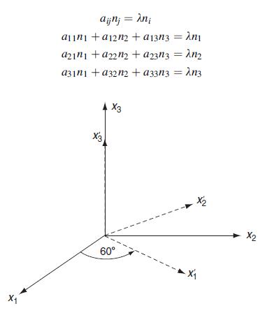
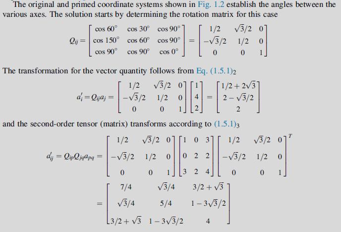
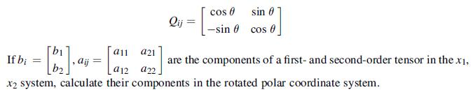
Determine the components of the vector bi and matrix aij given in Exercise 1.1 in a new coordinate system found through a rotation of 45° (π/4 radians) about the x1-axis. The rotation direction follows the positive sense presented in Example 1.2.Data from exercise 1.1For the given matrix/vector
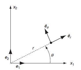
Consider the two-dimensional coordinate transformation shown in Fig. 1.8. Through the counterclockwise rotation q, a new polar coordinate system is created. Show that the transformation matrix for this case is given by:Fig 1.8 2 X2 e g r X
Show that the second-order tensor aδij, where a is an arbitrary constant, retains its form under any transformation Qij. This form is then an isotropic second-order tensor.
The most general form of a fourth-order isotropic tensor can be expressed by:where α, β, and γ are arbitrary constants. Verify that this form remains the same under the general transformation given by (1.5.1)5. + ; +

Showing 600 - 700 of 709

1
2
3
4
5
6
7
8

Step by Step Answers

Services

Sitemap
Fun
Definitions
Become Tutor
Used Textbooks
Study Help Categories
Recent Questions
Expert Questions
Campus Wear
Sell Your Books

Company Info

Security
Copyrights
Privacy Policy
Terms & Conditions
SolutionInn Fee
Scholarship
Online Quiz
Give Feedback, Get Rewards

Get In Touch

About Us
Contact Us
Career
Jobs
FAQ
Student Discount
Campus Ambassador

Secure Payment

Download Our App

© 2026 SolutionInn. All Rights Reserved