New Semester Started Get 50% OFF Study Help! --h --m --s Claim Now

Question Answers

Textbooks

Find textbooks, questions and answers

Oops, something went wrong!

Change your search query and then try again

Result Not Found

Books FREE
Study Help
Tutors
AI Study Planner NEW
Sell Books

Search
Sign In
Register

study help
engineering
elasticity theory applications

Elasticity Theory Applications And Numerics 4th Edition Martin H. Sadd Ph.D. - Solutions

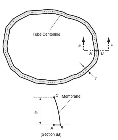
The example MATLAB code C.7 numerically integrated the integrals in solution (8.5.9) for the case of the flat rigid punch problem. Modify this example code to handle the case of the cylindrical punch given by solution (8.5.13) and thus generate the τ, max contours shown in Fig. 8.43.Equation
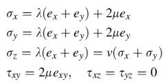
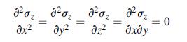
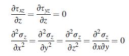
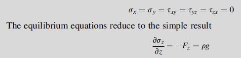
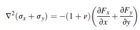
Under the assumption that σx = σy = τ, xy = 0, show that equilibrium and compatibility equations with zero body forces reduce to relations (9.1.2). Next integrate relations:to justify that σz = C1x + C2y + C3z + C4xz + C5yz + C6, where Ci are arbitrary constants.Equation 9.1.2 20, 20, 2, 2x2
During early development of the torsion formulation, Navier attempted to extend Coulomb’s theory for bars of circular section and to assume that there is no warping displacement for general cross-sections. Show that although such an assumed displacement field will satisfy all elasticity field
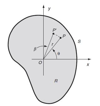
Referring to Fig. 9.2, if we choose a different reference origin that is located at point (a,b) with respect to the given axes, the displacement field would now be given by:where x and y now represent the new coordinates. Show that this new representation leads to an identical torsion formulation
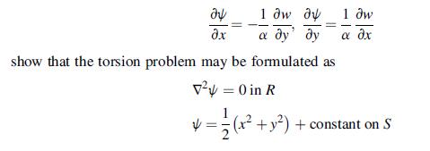
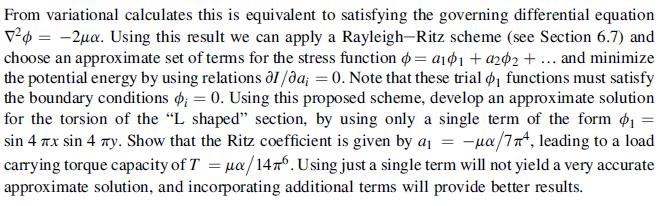
In terms of a conjugate functionΨ(x,y) defined by: 1 aw ay ' show that the torsion problem may be formulated as v =0 in R 24 x * = 1/2 (2 +1) 1 dw a dr + y) + constant on S
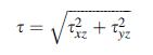
A function f(x,y) is defined as subharmonic in a region R if ∇2f ≥ 0 at all points in R. It can be proved that the maximum value of a subharmonic function occurs only on the boundary S of region R. For the torsion problem, show that the square of the resultant shear stress τ,2 = τ,2xz +
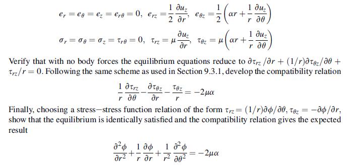
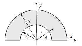
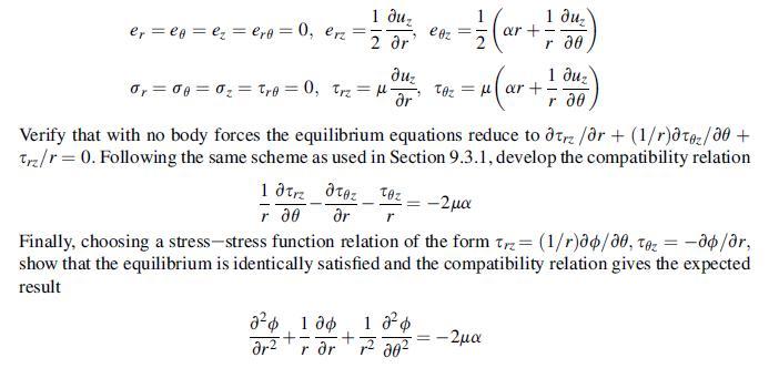
We wish to reformulate the torsion problem using cylindrical coordinates. First show that the general form of the displacements can be expressed as ur = 0, uθ = αrz, uz = uz(r,θ). Next show that this leads to the following strain and stress fields: er = e =e = ero = 0, erz 1 uz 2 dr' duz or=000
Using polar coordinates and the basic results of Exercise 9.6, formulate the torsion of a cylinder of circular section with radius a, in terms of the usual Prandtl stress function. Note for this case, there will be no warping displacement and ∅ = ∅(r). Show that the stress function is given
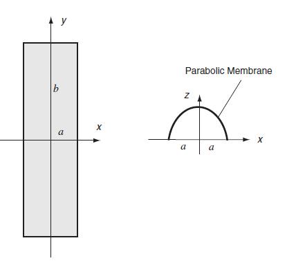
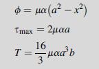
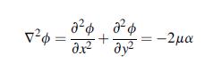
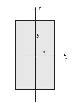
Employing the membrane analogy, develop an approximate solution to the torsion problem of a thin rectangular section as shown. Neglecting end effects at y =± b, the membrane deflection will then depend only on x, and the governing equation can be integrated to give z = ∅ = μα(a2 – x2), thus
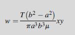
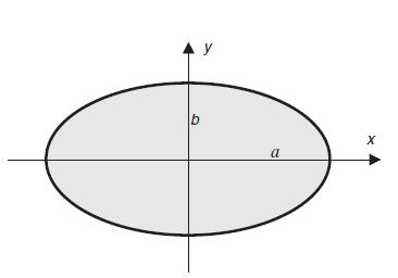
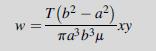
Using the stress results for the torsion of the elliptical section, formally integrate the strain-displacement relations and develop the displacement solution (9.4.11).Equation 9.4.11 W = T(b2 a2) XV
For the torsion of an elliptical section, show that the resultant shear stress at any point within the cross-section is tangent to an ellipse that passes through the point and has the same ratio of major to minor axes as that of the boundary ellipse.
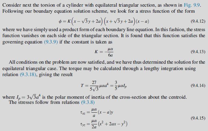
Develop relation (9.4.14) for the load-carrying torque of an equilateral triangular section.Equation 9.4.14 T= 27 3 Madt = sualp 5,3
For the torsion of a bar of elliptical section, express the torque equation (9.4.6) in terms of the polar moment of inertia of the section, and compare this result with the corresponding relation for the equilateral triangular section.Equation 9.4.6 T= 3b3 al +6
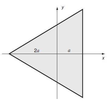
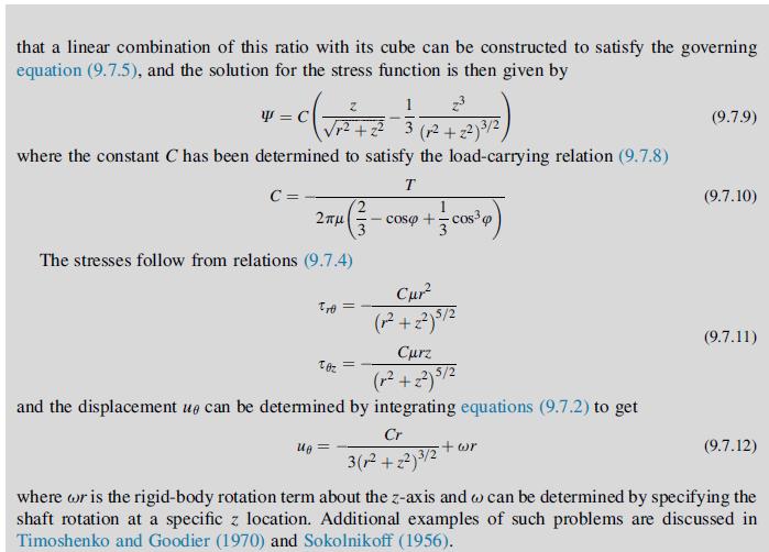
For the triangular section shown in Fig. 9.9, calculate the resultant shear stress along the line y = 0, and plot the result over the range –2a≤ x≤ a. Determine and label all maximum and minimum values.Fig 9.9 2a a X
For the triangular section of Example 9.2, plot contours of constant resultant shear stress:Point out how these contours would imply that the maximum shear stress occurs at the midpoints of each boundary side.Data from example 9.2 t=
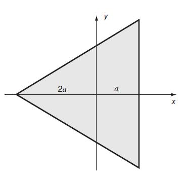
Consider the torsion of a bar of general triangular section as shown in the following figure. Using the boundary equation technique of Section 9.4, attempt a stress function solution of the form:where m1, m2, and a are geometric constants defined in the figure and K is a constant to be determined.
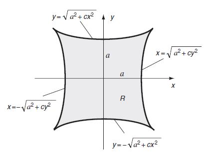
For the torsion problem in Example 9.3, explicitly justify that the required values for the constants appearing in the stress function are given by c = 3–√8 and K=–μα/[4a2(1–√2)]. Also calculate the resulting shear stresses and determine the location and value of the maximum stress.Data
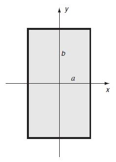
Attempt to solve the torsion of a rectangular section shown in Fig. 9.12 by using the boundary equation method. Show that trying a stress function created from the four products of the boundary lines x =± a and y=± b will not satisfy the governing equation (9.3.9).Fig 9.12Equation 9.3.9 b a X
Using the displacement formulation given in Section 9.3.2, use standard separation of variables to solve the torsion problem of an elliptical section shown in Fig. 9.7. For this problem it is only necessary to use results coming from the zero-separation constant case. Verify your solution with
Using the displacement formulation given in Section 9.3.2, use standard separation of variables to solve the torsion problem of a rectangular section shown in Fig. 9.12. Verify your solution with relation (9.5.14).Fig 9.12Equation 9.5.14 y b a X
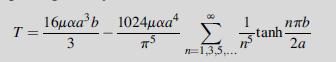
Using the torque relation (9.5.12) for the rectangular section, compute the nondimensional load-carrying parameter T/μαb4, and plot this as a function of the dimensionless ratio b/a over the range 1 ≤ b/a ≤10. For the case where b/a approaches 10, show that the load-carrying behavior can be
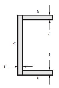
Using the relation (9.5.16), develop an approximate solution for the load-carrying torque of the channel section shown.Equation 9.5.16 a b b t
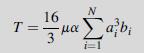
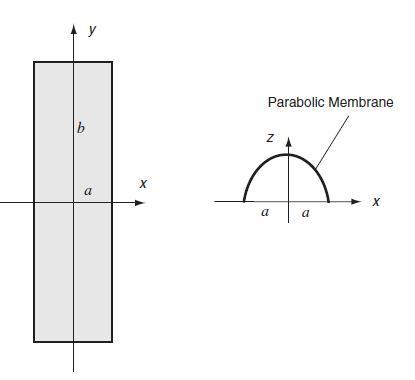
For the given narrow triangular section, show that the approximate torsional load carrying capacity is given by T = 2/3 μαc3oh. Use the parabolic membrane scheme outlined in Exercise 9.8 for any level y in the section.Data from exercise 9.8Employing the membrane analogy, develop an approximate
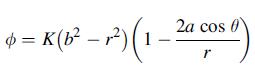
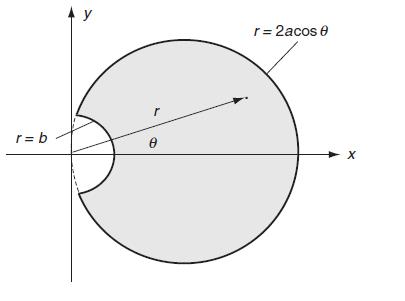
A circular shaft with a keyway can be approximated by the section shown in the following figure. The keyway is represented by the boundary equation r = b, while the shaft has the boundary relation r = 2a cos θ. Using the technique of Section 9.4, a trial stress function is suggested of the
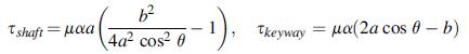
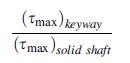
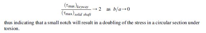
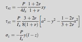
For the keyway section of Exercise 9.23, show that resultant stresses on the shaft and keyway boundaries are given by:Determine the maximum values of these stresses, and show that for b the maximum keyway stress is approximately twice that of the shaft stress. Finally, make a plotof the stress
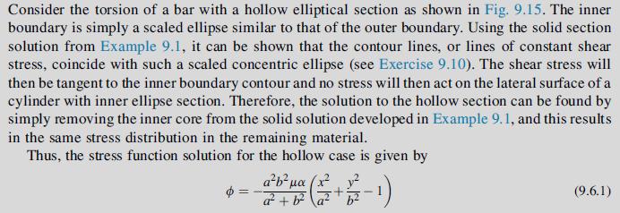
For the hollow elliptical section in Example 9.5, explicitly show that the given stress function (9.6.1) will yield the constant value specified by (9.6.2) on the inner boundary. Next using the methods from Example 9.1, show that the general torque relation (9.3.31) will also produce the result
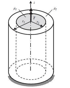
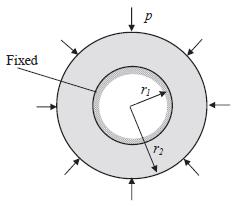
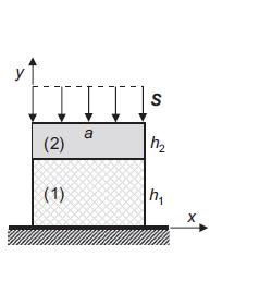
The illustrated uniform composite circular rod is composed of a solid inner core with shear modulus μ1 and a different outer core material of modulus μ2. The two materials are assumed to be perfectly bonded at interface r = r1, and thus the interfacial tangential displacements must be continuous
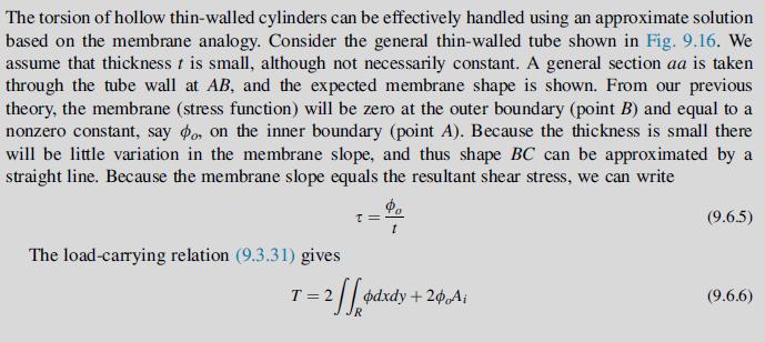
Example 9.6 provides the torsion solution of a closed thin-walled section shown in Fig. 9.16.Investigate the solution of the identical section for the case where a small cut has been introduced as shown in the following figure. This cut creates an open tube and produces significant changes to the
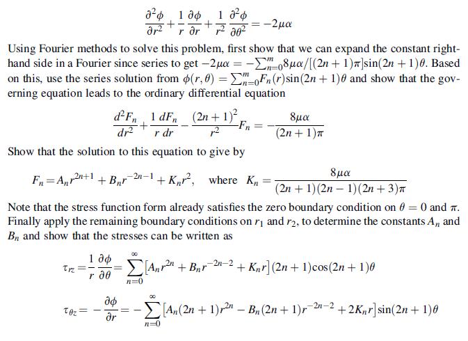
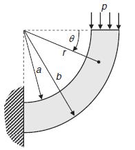
Consider the torsion of a rod with the half-ring cross-section as shown. Formulating the problem in polar coordinates (see Exercise 9.6), the governing stress function equation becomes:Data from exercise 9.6We wish to reformulate the torsion problem using cylindrical coordinates. First show that
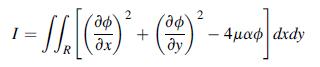
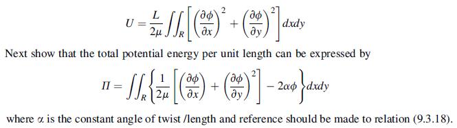
The potential energy per unit length for the torsion problem was given in Exercise 6.16. Using the principle of minimum potential energy, δ∏ = 0 and this leads to a minimization of the following integral expression: Data from exercise 6.16From Chapter 9 using the Saint-Venant formulation, the
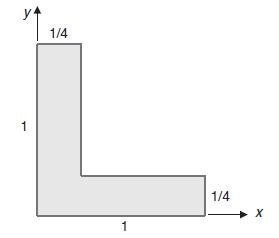
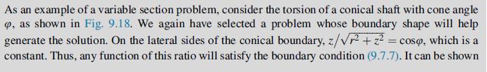
For the solution of the conical shaft given in Example 9.7, compare the maximum shearing stress τθz with the corresponding result from strength of materials theory. Specifically, consider the case with a cone angle φ = 20ᵒ with z = l, and compare dimensionless values of τθzl3/T.Data from
Make a comparison study of the torsion of a conical shaft given in Example 9.7 with corresponding results from mechanics of materials. First develop the τ θz shear stress relations for each theory, and then make a comparison plot of the maximum section shear stress (normalized by the torque, T)
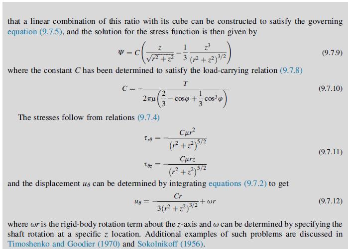
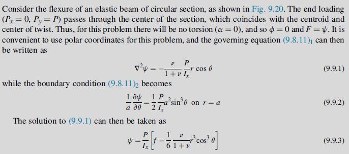
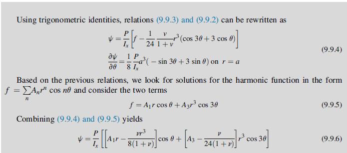
Determine the displacement field for the flexure problem of a beam of circular section given in Example 9.8. Starting with the stress solution (9.9.9), integrate the strain-displacement relations and use boundary conditions that require the displacements and rotations to vanish at z = 0. Compare
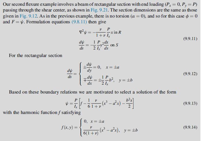
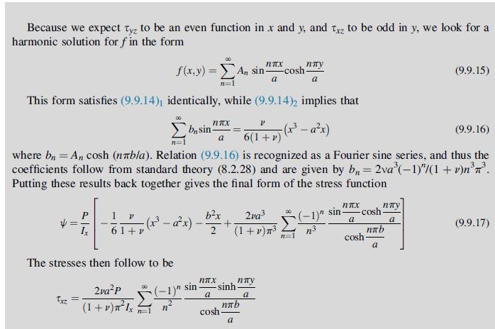
Make a comparison of theory of elasticity and strength of materials shear stresses for the flexure of a beam of rectangular section from Example 9.9. For each theory, calculate and plot the dimensionless shear stress τyz(0, y) b2/P versus y/b for an aspect ratio b/a = 1.Data from example 9.9 Our
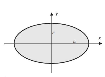
Solve the flexure problem without twist of an elastic beam of elliptical section as shown in Fig. 9.7 with Py = P. Show that the stress results reduce to (9.9.9) for the circular case with a = b.Fig 9.7Equation 9.9.9 a X
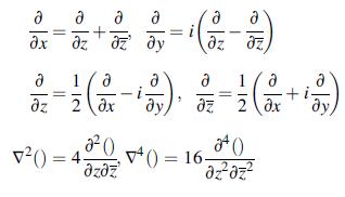
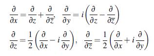
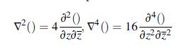
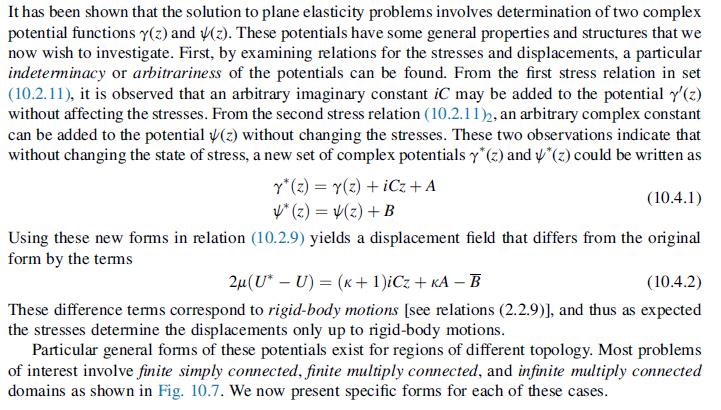
Derive the relations (10.1.4) and (10.2.5):Equation 10.1.4Equation 10.2.5 (3) = i (1/2- z z' z. Kz. x ( - ) a z 2 470 V()=4- z z dz 2 () = 16 24 (1) azaz +i- x
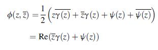
Formally integrate relation (10.2.6) and establish the result:Equation 10.2.6 (z, Z) = 1/2 (zy (z) + y (2) + V (2) + (2) Re(Zy(z)+(z))
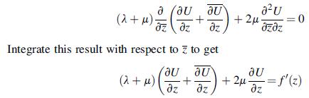
Starting with the Navier equations (10.2.2) for plane strain, introduce the complex displacement U = u + iv, and show that:where f′(z) is an arbitrary analytic function of z. Next, combining both the preceding equation and its conjugate, solve for ∂U/∂z, and simplify to get form
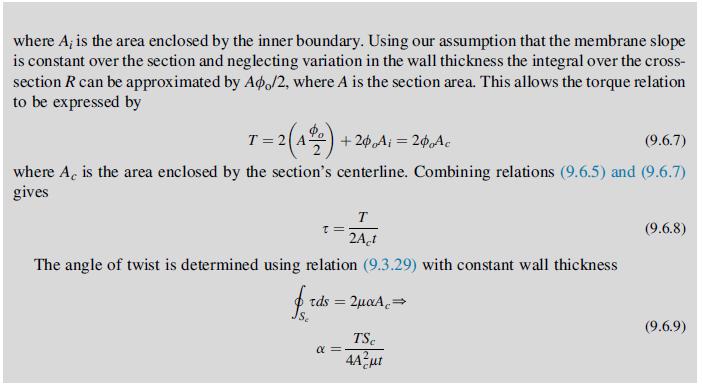
Establish the relations: [2(u +iv)] = [2Y(3) + (3)] = (ex - e + 2iexy) where ex, ey, and exy are the strain components.
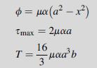
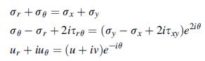
Explicitly derive the fundamental stress combinations: 0x + Oy = 2 [Y(2) + Y(2) Oy - Ox + 2itxy = 2[zy" (z)+(2)] Next solve these relations for the individual stresses 0x = 2 Re [y' (2) - 123v" (2) -124 (2)] 0,- 2 Rey(2) +- TY (2) + W(] Txy = Im [ZY" (2) + (z)]
Develop the polar coordinate transformation relations for the stress combinations and complex displacements given in equations (10.2.12).Equation 10.2.12 or +0g = 0x + ay ge-0, +2itre (ay-ax+2ity)e0 u, + iug = (u + iv)e-i =
Determine the Cartesian stresses and displacements in a rectangular domain (–a≤ x≤ a; – b≤y≤ b) from the potentials γ (z) = Aiz2,Ψ(z) =–Aiz2, where A is an arbitrary constant. Discuss the boundary values of these stresses, and show that this particular case could be used to solve a
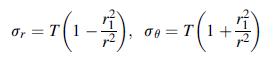
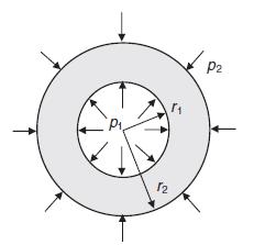
Determine the polar coordinate stresses corresponding to the complex potentials γ (z) = Az and Ψ(z) = Bz–1, where A and B are arbitrary constants. Show that these potentials could solve the plane problem of a cylinder with both internal and external pressure loadings.
Show that the potentials γ (z) = 0,Ψ(z) = A/z will solve the problem of a circular hole of radius a with uniform pressure loading p in an infinite elastic plane. Determine the constant A and the stress and displacement fields for r ≥ a.
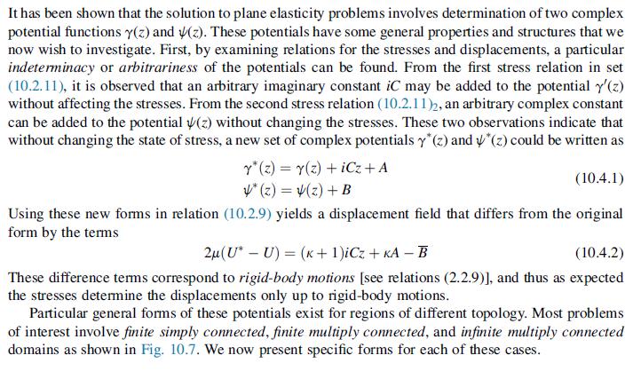
Consider the problem geometry described in Exercise 10.9. Show that the suggested potentials (with different A) can also be used to solve the problem of a rigid inclusion of radius a + δ, which is forced into the hole of radius a. Determine the new constant A and the stress and displacement fields
From Section 10.4, the complex potentials:would be the appropriate forms for a problem in which the body contains a hole surrounding the origin (i.e., multiply connected). Show for this case that the complex displacement U is unbounded as IzI→0 and IzI→∞. Also, explicitly verify that the
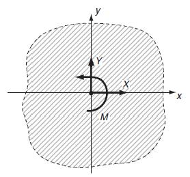
Show that the resultant moment caused by tractions on a boundary contour AB is given by relation (10.3.2):Equation 10.3.2 B M = Re[x(z) - z(z) zzy' (2), where x' (2) = 4(z)
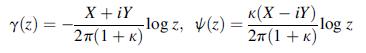
An infinite elastic medium IzI ≥ a is bonded over its internal boundary IzI =a to a rigid inclusion of radius a. The inclusion is acted upon by a force X + iY and a moment Mabou its center. Show that the problem is solved by the potentials: Y(z) = = Uo X +iY 2(1+K) X-iY 2(1+K) -log z -K log z + X
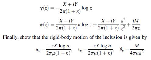
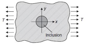
An infinite isotropic sheet contains a perfectly bonded, rigid inclusion of radius a and is under uniform tension T in the x-direction as shown. Show that this problem is solved by the following potentials:Note that because of the problem symmetry, the inclusion will not move. In solving this
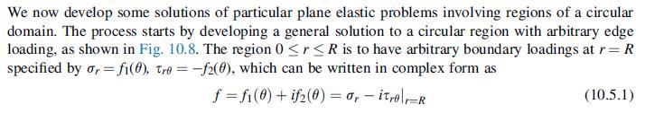
Consider the unit disk problem with displacement boundary conditions ur + iuθ = h(ς) on C: ς = eiθ. Using Cauchy integral methods described in Section 10.5, determine the form of the potentials γ (z) and Ψ(z).Data from section 10.5 We now develop some solutions of particular plane elastic
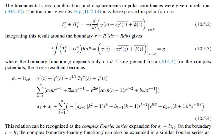
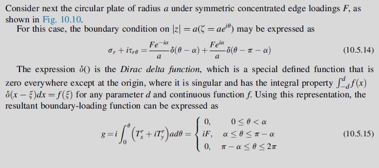
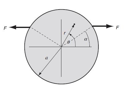
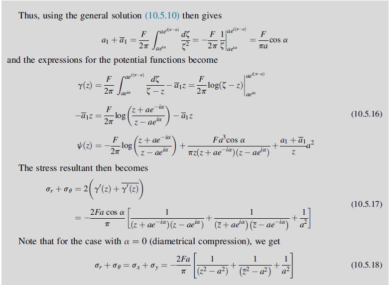
For Example, 10.3 with α = 0, verify that the stresses from equation (10.5.18) reduce to those previously given in Eq. (8.4.69).Data from example 10.3Equation 10.5.18Equation 8.4.69 Consider next the circular plate of radius a under symmetric concentrated edge loadings F, as shown in Fig. 10.10.
Consider the concentrated force system problem shown in Fig. 10.11. Verify for the special case of X = P and Y = M = 0 that the stress field reduces to relations (10.6.5). Also determine the corresponding stresses in polar coordinates.Fig 10.11Equation 10.6.5 F M +
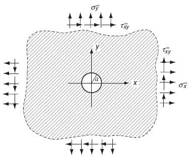
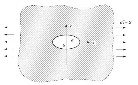
For the stress concentration problem shown in Fig. 10.14, solve the problem with the far field loadings σ∞x = σ∞y = S; τ ∞xy = 0, and compute the stress concentration factor. Verify your solution with that given in Eqs. (8.4.9) and (8.4.10).Fig 10.14Equation 8.4.9Equation 8.4.10 oy txy X
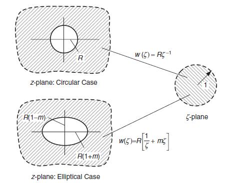
Verify the mappings shown in Fig. 10.16 by explicitly investigating points on the boundaries and the point at infinity in the z-plane.Fig 10.16 I R z-plane: Circular Case R(1-m) R(1+m) z-plane: Elliptical Case w (5)= R5-1 W(5)=R + m 5-plane
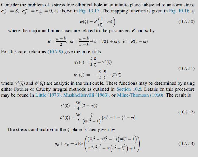
Consider relation (10.7.14) for the circumferential stress σφ on the boundary of the elliptical hole shown in Fig. 10.17. Explicitly verify that the maximum stress occurs at φ = π/2. Next plot the distribution of σφ versus φ for the cases of m = 0, ± 0.5, ± 1.Fig 10.17Equation 10.7.14 b
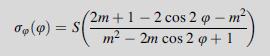
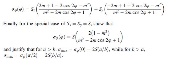
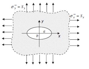
Using the solution from Example 10.7, apply the principle of superposition and solve the problem of a stress-free elliptical hole under uniform biaxial tension as shown. In particular show that the circumferential stress is given by:Data from example 10.7 Jp (9) = Sx (2m+1-2 cos 2p - m m 2m cos
Consider the problem of an infinite plate containing a stress-free elliptical hole withσ∞x = σ∞y = 0; τ∞xy = S. For this problem, the derivative of the complex potential has been developed by Milne-Thomson (1960): 22- W S! dz (5)^p
Verify the crack-tip stress distributions given by Eqs. (10.8.6) and (10.8.7).Equation 10.8.6Equation 10.8.7 2Sa 2ar Oy - 0x + 2ity = 0x + ay: 0 COS 2 30 sino(+cos) sin cos 2Sa 2ar 30 2
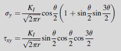
Construct a contour plot of the crack tip stress component σy from Eq. (10.8.7). Normalize values with respect to KI.Equation 10.8.7 try = K 2r Cos K 2r 0 / (1+ sin-sin 0 0 30 -sin-cos-cos cos 2 30
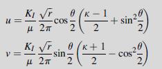
Verify that the crack-tip displacements are given by Eq. (10.8.8).Equation 10.8.8 u= v= KI r 8 (K. - cos 2 Ki r K 2 sin 1/1(-2 + 0 (K IN x+1 2 2 + sin - cos
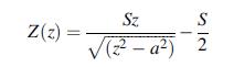
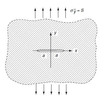
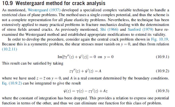
Show that the Westergaard stress function:with A = S/2 solves the central crack problem shown in Fig. 10.19.Fig 10.19 Z(z) Sz (2-a) 2 NIS
Following similar procedures as in Section 10.9, establish a Westergaard stress function method for skew-symmetric crack problems. For this case, assume that loadings are applied skew-symmetrically with respect to the crack, thereby establishing that the normal stress σy vanishes along y = 0. Show
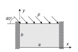
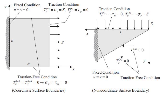
Using Cartesian coordinates, express all boundary conditions for each of the illustrated problems.a. b.c. d.e. f. 40% a
Using polar coordinates, express all boundary conditions for each of the illustrated problems.a. b. c. d. e. f. P, 12 " P
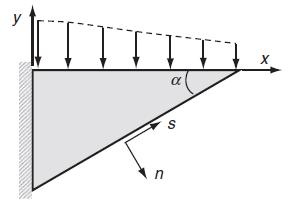
The tapered cantilever beam shown in the following figure is to have zero tractions on the bottom inclined surface. As discussed in the text (see Fig. 5.4 ), this may be specified by requiring Tx (n) = T(n)y = 0. This condition can also be expressed in terms of components normal and tangential to
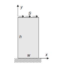
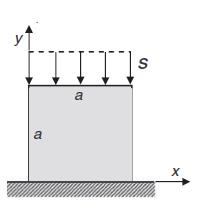
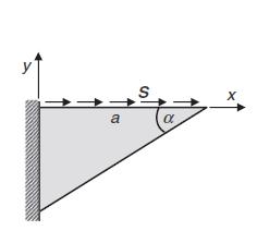
The following two-dimensional problems all have mixed boundary conditions involving both traction and displacement specifications. Using various field equations, formulate all boundary conditions for each problem solely in terms of displacements.a. b. TITI a a S X
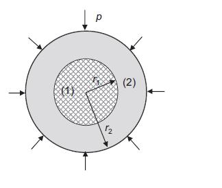
For problems involving composite bodies composed of two or more materials, the elasticity solution requires both boundary conditions and interface conditions between each material system. The solution process is then developed independently for each material by satisfying how the various material
Solve Exercise 5.5 using slip interface conditions, where the normal components of displacement and traction are continuous, the tangential traction vanishes, and the tangential displacement can be discontinuous.Data from exercise 5.5For problems involving composite bodies composed of two or more
As mentioned in Section 5.6, Sainte-Venant’s principle will allow particular boundary conditions to be replaced by their statically equivalent resultant. For problems (b), (c), (d),and (f) in Exercise 5.1, the support boundaries that had fixed displacement conditions can be modified to specify
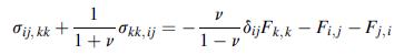
Go through the details and explicitly develop the Beltramie-Michell compatibility equations (5.3.3).Equation 5.3.3 Dij, kk + l 1 - Okk,ij = - + v -1 V - 6jFk,k - Fij - Fj,i 1 - v
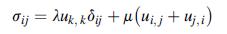
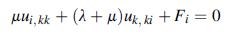
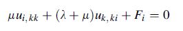
For the displacement formulation, use relations (5.4.1) in the equilibrium equations and develop the Navier equations (5.4.3).Equation 5.4.1Equation 5.4.3 ;; = , + {ui,j + 1;;)
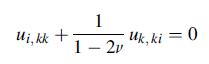
For the general displacement formulation with no body forces, show that Navier’s equations(5.4.3) reduce to the form:and thus, the field equation formulation will now only depend on the single elastic constant, Poisson’s ratio. For the case with only displacement boundary conditions, this fact
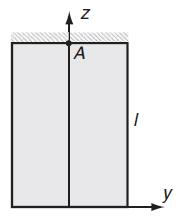
Carry out the integration details to develop the displacements (5.7.4) in Example 5.1.Equation 5.7.4Data from example 5.1As an example of a simple direct integration problem, consider the case of a uniform prismatic bar stretched by its own weight, as shown in Fig. 5.11. The body forces for this
Using the inverse method, investigate which problem can be solved by the two-dimensional stress distribution σx = Axy, τ xy = B + Cy2, σy = 0, where A, B, and C are constants. First show that the proposed stress field (with zero body force) satisfies the stress formulation field equations under
Show that the following stress components satisfy the equations of equilibrium with zero body forces, but are not the solution to a problem in elasticity: ox = c[y +v(x - y)] oy = c[x +v(y-x)] 0 = cv(x + y) Txy = -2cvxy Tyz = Tzx = 0, c = constant #0
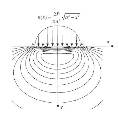
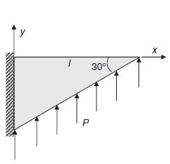
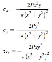
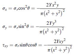
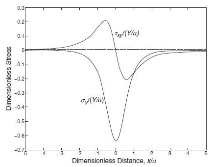
Consider the problem of a concentrated force acting normal to the free surface of a semi-infinite solid as shown in case: (a) of the following figure. The two-dimensional stress field for this problem is given by equations (8.4.36) as:Equation 8.4.36Using this solution with the method of
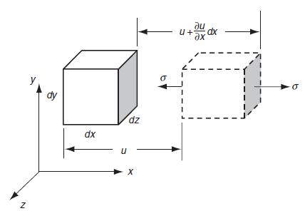
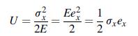
The uniaxial deformation case as shown in Fig. 6.1 was used to determine the strain energy under uniform stress with zero body force. Determine this strain energy for the case in which the stress varies continuously as a function of x and also include the effect of a body force Fx. Neglecting
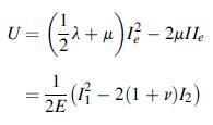
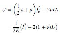
Since the strain energy has physical meaning that is independent of the choice of coordinate axes, it must be invariant to all coordinate transformations. Because U is a quadratic form in the strains or stresses, it cannot depend on the third invariants IIIe or I3, and so it must depend only on
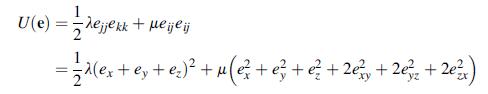
Starting with the general expression (6.1.7), explicitly develop forms (6.1.9) and (6.1.10) for the strain energy density.Equation 6.1 .7Equation 6.1 .9Equation 6.1 .10 U = 2(0xex + yey + orez + Exy Yay +Tyz Yyz + TexYx): 1 zije ij
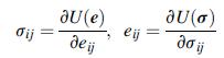
Differentiate the general three-dimensional isotropic strain energy form (6.1.9) to show that:Equation 6.1 .9 dij aU(e) ij
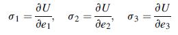
For the isotropic case, express the strain energy function in terms of the principal strains, and then by direct differentiation show that: 01 au ' 02 au z' 03 au
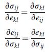
Using equations (6.1.12), develop the symmetry relations (6.1.13), and use these to prove the symmetry in the elasticity tensor Cijkl = Cklij.Equation 6.1 .12Equation 6.1 .13 dij aU(e) ij eij aU(a) ;
For the general anisotropic case withσij = Cijklekl assuming that Cijkl = Cklij show thatσij = ∂U(e)/∂eij.
In light of Exercise 6.2 , consider the formulation where the strain energy is assumed to be a function of the two invariants U = U(Ie, IIe). Show that using the relation σij = ∂U/∂eij and employing the chain rule, yields the expected constitutive law (4.2.7).Equation 4.2 .7Data from exercise
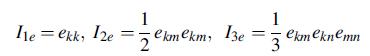
Consider the case of a nonlinear elastic material, and extend Exercise 6.8 for the case where the strain energy depends on three invariants of the strain tensor U = U(I1e, I2e, I3e), where:Note that this new choice of invariants does not change any fundamental aspects of the problem.Show that using
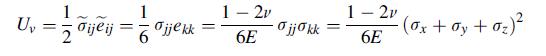
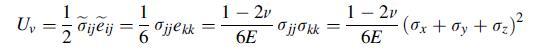
Verify the decomposition of the strain energy into volumetric and deviatoric parts as given by equations (6.1.16) and (6.1.17).Equation 6.1 .16Equation 6.1 .17 1 U = - = 1/ dijeij 2 o jje kk 1-2v 6E -jjkk = 1 - 2v 6E (0x + ay +0)
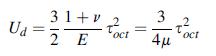
Starting with relations (6.1.16) and (6.1.17), show that the volumetric and distortional strain energies can be expressed in terms of the invariants of the stress matrix as:Equation 6.1 .16Equation 6.1 .17Results from Exercise 6.10 may be helpful.Data from exercise 6.10 Verify the decomposition of
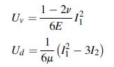
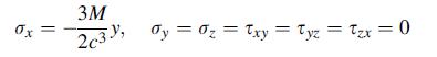
Show that the distortional strain energy given by (6.1.17) is related to the octahedral shear stress (3.5.4)2 by the relation:Equation 6.1 .17Equation 3.5 .4Results from Exercise 3.5 may be helpful.Data from exercise 3.5 A two-dimensional state of plane stress in the x, y-plane is defined byσz =
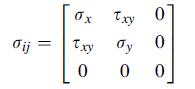
A two-dimensional state of plane stress in the x,y-plane is defined by the stress matrix:Determine the strain energy density for this case in terms of these nonzero stress components. Ox Txy Tij Txy Ty 0 0 0 0 0
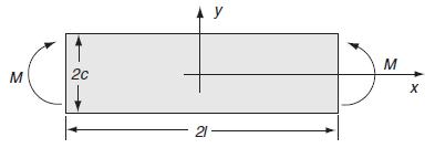
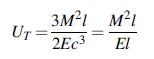
The stress field for a beam of length 2l and depth 2c under end bending moments M (see Fig. 8.2) is given by:Fig 8.2Determine the strain energy density and show that the total strain energy in the beam is given by:where I is the section moment of inertia. Assume unit thickness in the z-direction.
The stress field for the torsion of a rod of circular cross-section is given by:where α is a constant and the z-axis coincides with the axis of the rod. Evaluate the strain energy density for this case, and determine the total strain energy in a rod with section radius R and length L. 0x = 0 = 0 =
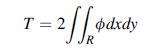
From Chapter 9 using the Saint-Venant formulation, the stress field for the torsion of rod of general cross-section R can be expressed by:where ∅ = ∅(x, y) is the Prandtl stress function. Show that the total strain energy in a rod of length L is given by:Equation 9.3 .18 dx = 0y = 0z = txy = 0,
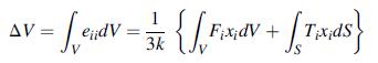
Using the reciprocal theorem, choose the first state as ui(1)= Axi; Fi(1)= 0; Ti(1) = 3kAni, and take the second state as ui, Fi, Ti to show that the change in volume of the body is given bywhere A is an arbitrary constant and k is the bulk modulus. AV= * = [ endv = 3} / { / Fix;dv + [ Tixids} 3k
Rework Example 6.2 using the trigonometric Ritz approximation wj = sin jπx/l. Develop a two-term approximate solution and compare it with the displacement solution developed in the text. Also compare each of these approximations with the exact solution (6.7.9) at midspan x = l/2.Data from example
Using the bending formulae (6.6.9), compare the maximum bending stresses from the cases presented in Example 6.2 and Exercise 6.18 . Numerically compare these results with the exact solution; see (6.7.9) at midspan x = l/2.Data from example 6.2Consider a simply supported Euler-Bernoulli beam of
Invert the plane strain form of Hooke’s law (7.1.3) and express the strains in terms of the stresses as:Equation 7.13 ex ey v = 1 + ((1 v ox - vy] E exy 1+v E -[(1 v)oy - vox] 1 + v E -Txy
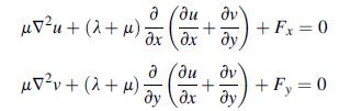
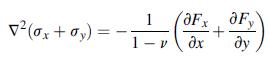
For the plane strain case, develop Navier equations (7.1.5) and the BeltramieMichell compatibility relation (7.1.7).Equation 7.1 .5Equation 7.1 .7 / v uTu+ (2+ ) + uT2v + (1 + ) + + Fx = 0 +Fy=0
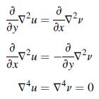
Verify the following relations for the case of plane strain with constant body forces: a 12 a -1u 4 = x 2 12 4v=0
At the end of Section 7.1 , it was pointed out that the plane strain solution to a cylindrical body of finite length with zero end tractions could be found by adding a corrective solution to remove the unwanted end loadings being generated from the axial stress relationσz = v(σx + σy). Using
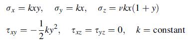
In the absence of body forces, show that the following stresses:satisfy the plane strain stress formulation relations. 0x = kxy, 0y = kx, 0=vkx(1+y) 1 ky, Txz = Tyz = 0, k = constant Txy

Showing 500 - 600 of 709

1
2
3
4
5
6
7
8

Step by Step Answers

Services

Sitemap
Fun
Definitions
Become Tutor
Used Textbooks
Study Help Categories
Recent Questions
Expert Questions
Campus Wear
Sell Your Books

Company Info

Security
Copyrights
Privacy Policy
Terms & Conditions
SolutionInn Fee
Scholarship
Online Quiz
Give Feedback, Get Rewards

Get In Touch

About Us
Contact Us
Career
Jobs
FAQ
Student Discount
Campus Ambassador

Secure Payment

Download Our App

© 2026 SolutionInn. All Rights Reserved