New Semester Started Get 50% OFF Study Help! --h --m --s Claim Now

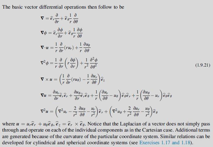
Question Answers

Textbooks

Find textbooks, questions and answers

Oops, something went wrong!

Change your search query and then try again

Result Not Found

Books FREE
Study Help
Tutors
AI Study Planner NEW
Sell Books

Search
Sign In
Register

study help
engineering
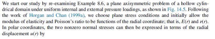
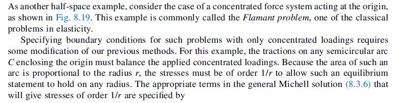
elasticity theory applications

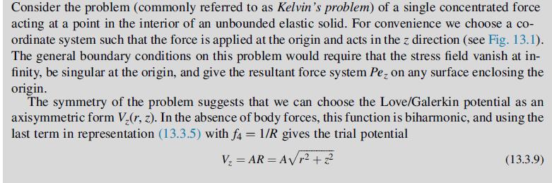
Elasticity Theory Applications And Numerics 4th Edition Martin H. Sadd Ph.D. - Solutions

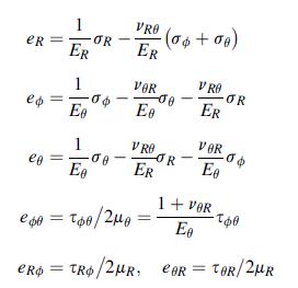
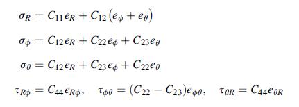
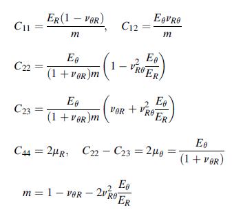
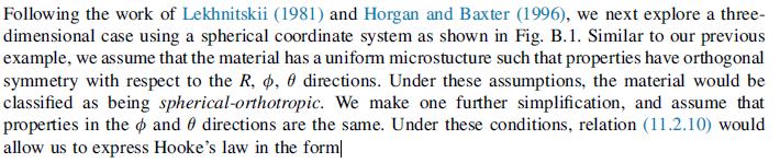
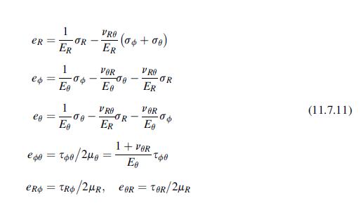
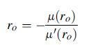
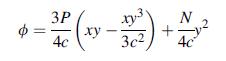
For the spherically orthotropic problem, justify that Hooke’s law (11.7.11) can be inverted into form (11.7.13) under the relations (11.7.14).Equation 11.7.11Equation 11.7.13Equation 11.7.14 eR ed eo ER 1 Ee OR VRO . ER VOR Ee (06 +00) e40 = too/2g = eR$ = TRO/2R, -JA ----- VRO ER 1 + VOR Ee OR
Under the stated symmetry conditions in Section 11.7.2, explicitly show that in the absence of body forces the general equilibrium equations reduce to forms (11.7.17) and (11.7.18).Verify the general displacement solution given by (11.7.19) and (11.7.20), and the particular stress solution
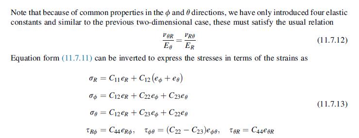
For the rotating disk problem given previously in Example 8.11, the governing equilibrium equation was given by (8.4.74). Since this equation is also valid for anisotropic materials, consider the polar-orthotropic case and use equations (11.7.3) to express the equilibrium equation in terms of the
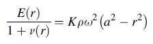
Using the results from Exercise 11.27, show that the stresses in a rotating solid circular polar-orthotropic disk of radius a with boundary condition σr (a) = 0 are given by:Data from exercise 11.27For the rotating disk problem given previously in Example 8.11, the governing equilibrium equation
Consider the cantilever beam problem shown previously in Exercise 8.2 with no axial force (N =0). Assume a plane stress anisotropic model given by Hooke’s law (11.5.1) and governed by the Airy stress function equation (11.5.6). Show that the stress function:Next show that these stresses satisfy
Using the assumption for isotropic materials that a temperature change produces isotropic thermal strains of the form α(T– To)δij, develop relations (12.1.6).Equation 12.1.6 ij = kkoij + 2e - (31+2)a(T-To) dij 1+v eij E V dij Okkdij +a(TTo)dij E
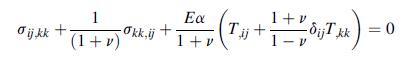
For the general three-dimensional thermoelastic problem with no body forces, explicitly develop the Beltrami-Michell compatibility equations: Tij kk + 1 -kk,ij + (1 + v) Ea 1+v Tij 1+v + 1 + OUTk 1-v -ijTkk) = 0
If an isotropic solid is heated nonuniformly to a temperature distribution T(x,y,z) and the material has unrestricted thermal expansion, the resulting strains will be eij = αTδ. Show that this case can only occur if the temperature is a linear function of the coordinates: T = ax + by+ cz + d
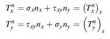
Express the traction boundary condition (12.3.8) in terms of displacement and temperature for the plane stress problem.Equation 12.3.8 T = Oxnx + xyny = (Tr), T" = Txynx + ayny
Develop the compatibility equations for plane strain (12.3.7) and plane stress (12.3.13).Equation 12.3.7Equation 12.3.13 12(ox toy) + (. 1-v _v?T= 0
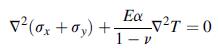
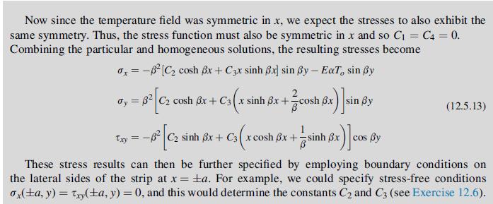
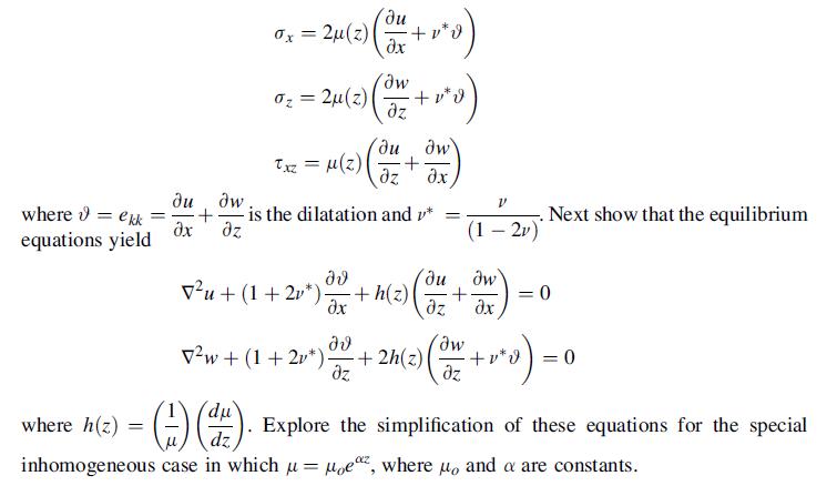
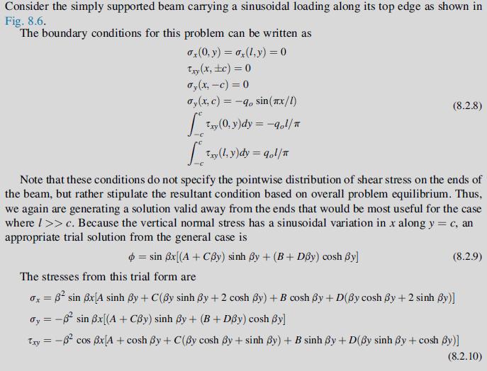
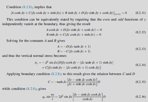
Explicitly develop the stress field Eq. (12.5.13) in Example 12.1 and determine the constants C2 and C3 for the case of stress-free edge conditions. Plot the value of σy through the thickness (vs. coordinate x) for both high-temperature (sin βy = 1) and low-temperature (sin βy
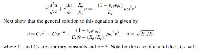
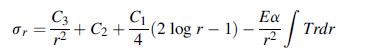
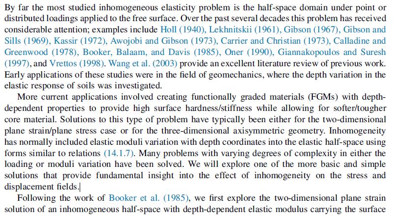
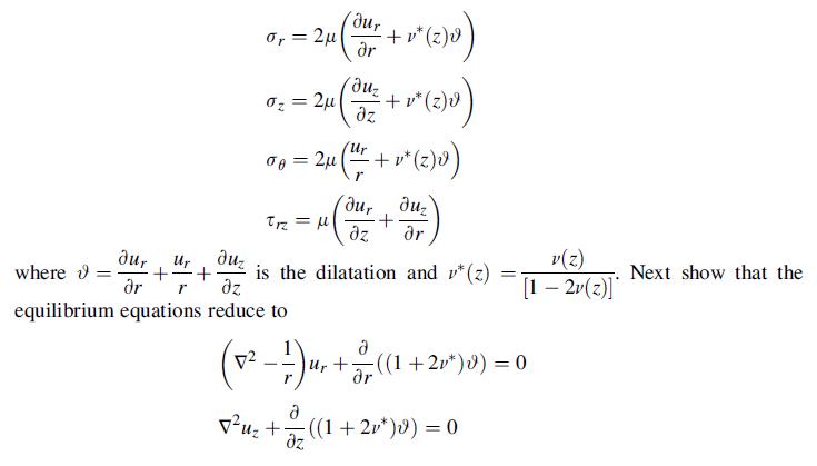
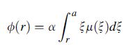
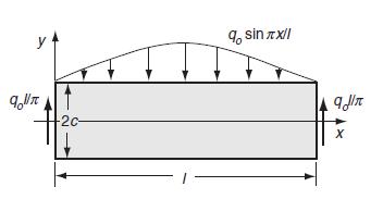
For the radially symmetric case, verify that the governing stress function equation can be expressed as (12.7.2). Integrate this equation and verify the general solution (12.7.4).Equation 12.7.2Equation 12.7.4 = 0= r dr + Ea-. (2) PI r drdr + + { [ ( ^ ) ; ] } ? P PI $= 0= r dr + Ea-. (2) PI r drdr + + { [ ( ^ ) : ] } ? P PI$
Verify the equilibrium equation in terms of displacement (12.7.5) for the radially symmetric case and then develop its general solution (12.7.6).Equation 12.7.5Equation 12.7.6 d [1 d dr r dr dT +/- (ru) ] = (1 +v) =/ dr
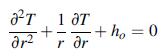
Consider the axisymmetric plane strain problem of a solid circular bar of radius a with a constant internal heat generation specified by ho. The steady-state conduction equation thus becomes:Using boundary condition T (a) = To, determine the temperature distribution, and then calculate the
Using the general displacement solution, solve the thermoelastic problem of a solid circular elastic plate with a restrained boundary edge at r = a. For the case of a uniform temperature distribution, show that the displacement and stress fields are zero.
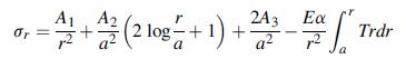
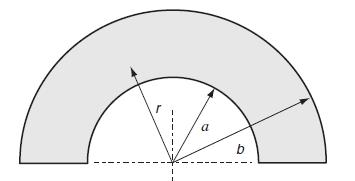
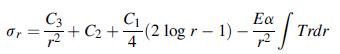
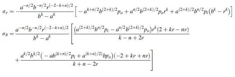
Consider the thermal stress problem in a circular ring as shown in the figure. Assuming the temperature and stress fields depend only on the radial coordinate r, the general solution is given by (12.7.4). If the surfaces r = a and r = b are to be stress free, show that the solution can be written
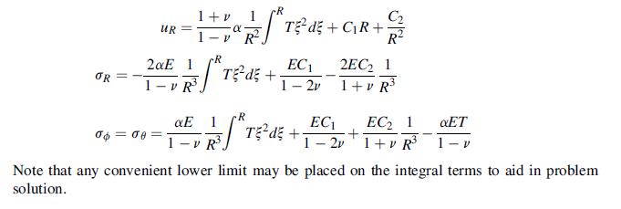
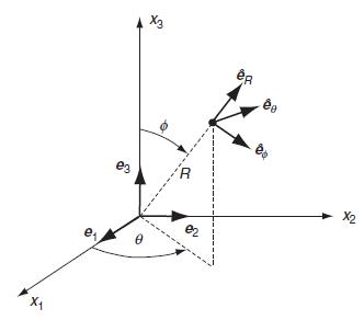
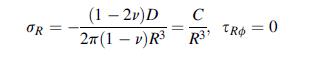
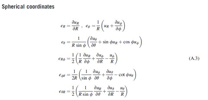
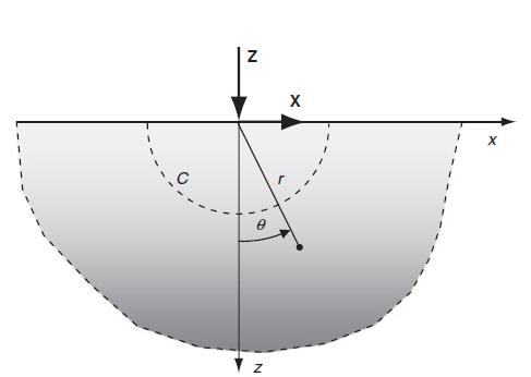
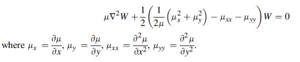
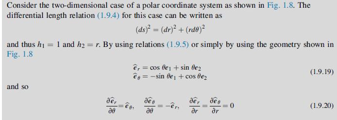
Consider the thermoelastic problem in spherical coordinates (R, ∅, θ); see Fig. 1.6. For the case of spherical symmetry where all field quantities depend only on the radial coordinate R, develop the general solution:Fig 1.6 OR = 1 C MR = 1 + 2/ *TedE+ CR + 2/ UR R 2E -R 1-VR^ Td +- 06 = 08=
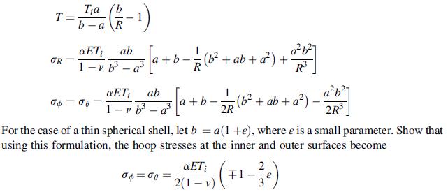
Use the general solution of Exercise 12.12 to solve the thermal stress problem of a hollow thick-walled spherical shell (a ≤ R≤b) with stress-free boundary conditions. Assuming that the problem is steady state with temperature conditions T(a) = Ti, T (b) = 0, show that the solution
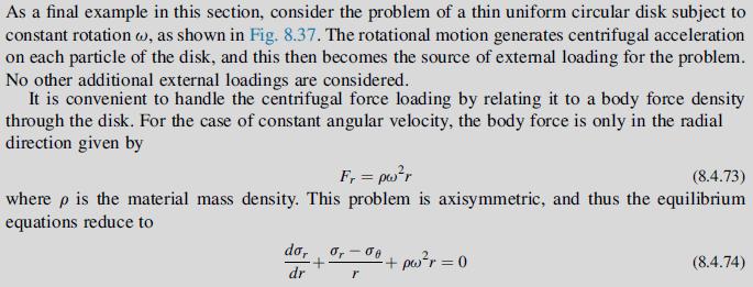
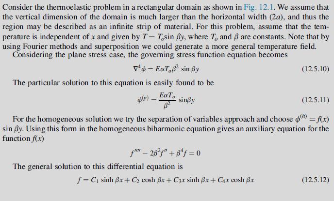
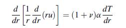
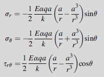
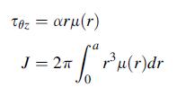
Explicitly develop relations (12.8.6) and verify that by using the value of b given in (12.8.7) the temperature terms will drop out of these relations.Equation 12.8.6Equation 12.8.7 0x = Jy = 2 du dv + dy Txy = 'du' dv + x du' dv - (+) +2- + [2B(2+u) - a(3 +2)]T du' x v' +2+ [2B(2+) - (3 +2)]T
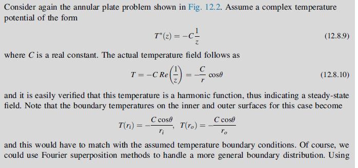
For Example 12.3, verify that the potentials γo(z), Ψo(z) given by relations (12.8.14) satisfy the stress-free boundary conditions on the problem.Data from example 12.3Equation 12.8.14 Consider again the annular plate problem shown in Fig. 12.2. Assume a complex temperature potential of the form
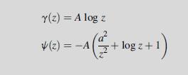
Using separation of variables and Fourier methods, solve the conduction equation and verify that the temperature distribution (12.8.20) in Example 12.4 does indeed satisfy insulated conditions on the circular hole and properly matches conditions at infinity.Equation 12.8.20Data from example 12.4 7,
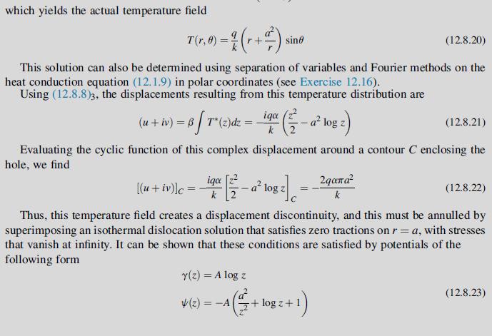
For Example, 12.4, explicitly develop the stresses (12.8.25) from the complex potentials given by Eq. (12.8.23).Equation 12.8.23Equation 12.8.25Data from example 12.4 Y(z) = A log z (2) = 4 (4/2 -A +1) +log z +1
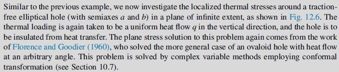
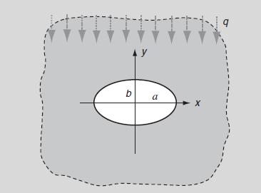
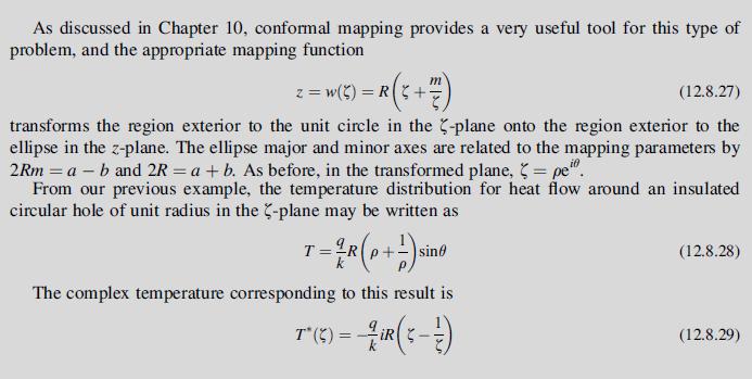
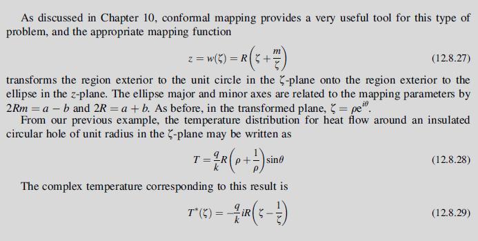
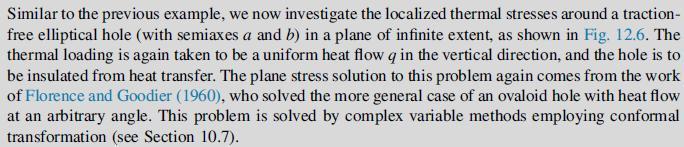
Plot the isotherms (contours of constant temperature) for Examples 12.4 and 12.5.Data from example 12.5Data from example 12.4 Similar to the previous example, we now investigate the localized thermal stresses around a traction- free elliptical hole (with semiaxes a and b) in a plane of infinite
For the elliptical hole problem in Example 12.5, show that by letting m = 0, the stress results will reduce to those of the circular hole problem given in Example 12.4.Data from example 12.5Data from example 12.4 Similar to the previous example, we now investigate the localized thermal stresses
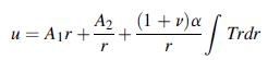
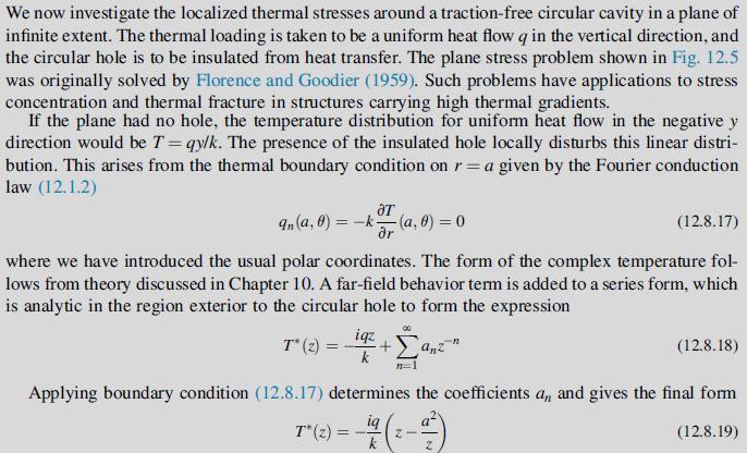
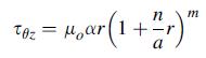
In Example 12.5, show that the dimensionless hoop stress around the boundary of the hole is given by:Data from example 12.5 Je e Exqa/k For the cases m = (1 +m)[(1 +m+m) sine -msin30] (1-2m cos20+ m) = 0, 1/2, 1, plot and compare the behaviour of 7 versus 0 (0 0 2).
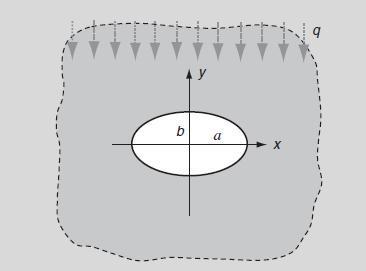
Show that for the plane anisotropic problem, the heat-conduction equation for uncoupled steady-state conditions is given by:Looking for solutions that are of the form T = (x+λy), show that this leads to the quadratic characteristic equation:Using the fact that kxxkyy > k2xy, demonstrate that
Using the Helmholtz representation, determine the displacement field that corresponds to the potentials∅ = x2 + 4y2, φ = R2e3. Next show that this displacement field satisfies Navier’s equation with no body forces.
Explicitly show that the dilatation and rotation are related to the Helmholtz potentials through relations (13.1.3).Equation 13.1.3 1 0 = ekk = ikky @j = = 2 Pi,kk
For the case of zero body forces, show that by using the vector identity (1.8.5)9 Navier’s equation can be written as:Using repeated differential operations on this result, show that the displacement vector isbiharmonic. Furthermore, because the stress and strain are linear combinations of first
For the case of Lame´’s potential, show that strains and stresses are given by (13.2.3).Equation 13.2.3 eij - 2 Tj = 0jj
Justify that the Galerkin vector satisfies the governing equation (13.3.2).Equation 13.3.2 VV= F 1-v
Show that the Helmholtz potentials are related to the Galerkin vector by relations (13.3.3).Equation 13.3.3 1 - 2v 2. -(V.V), 1-v (.)
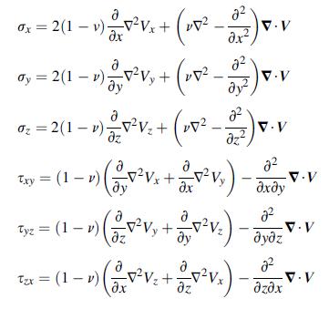
Justify relations (13.3.4) for the stress components in terms of the Galerkin vector.Equation 13.3.4 1-4 (20-240) +125 - (1-1)2-0 = 1-4 (-41) +1,4(-1)2=60 1-4 (/0 - (44) + 1,4 (1-1)2 = 0 D Try - (1-1) (1,00 + 0x). - Tyz = (1 v) (2 27V. - ax 2 (2 27V, + 3y VV ) - ayz Tax = (1 - 1) (2 x VV + 0 2 0
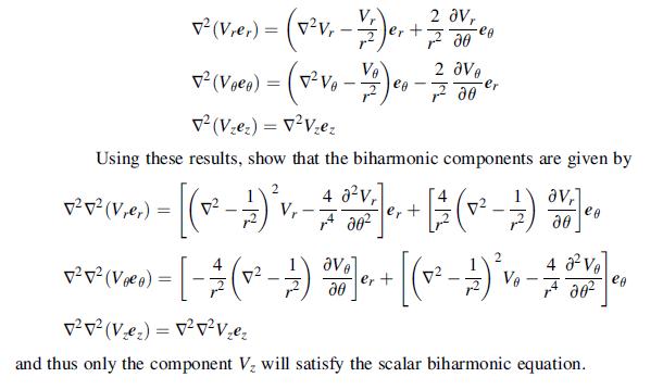
For the case of zero body forces, the Galerkin vector is biharmonic. However, it was pointed out that in curvilinear coordinate systems, the individual Galerkin vector components might not necessarily be biharmonic. Consider the cylindrical coordinate case where V = Vrer + Vθeθ + Vzez. Using the
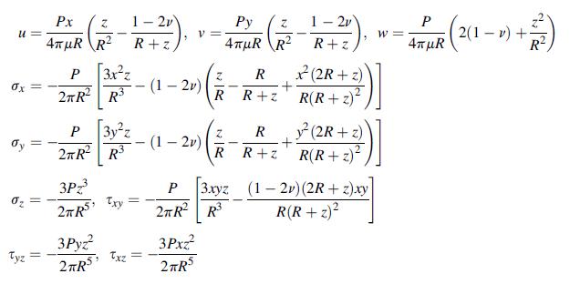
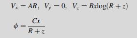
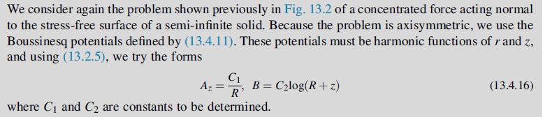
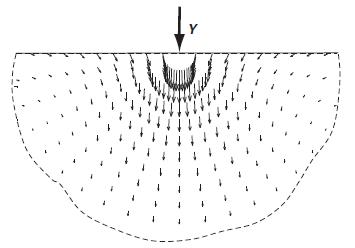
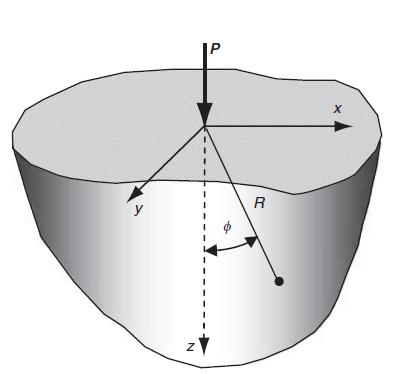
Explicitly show that Boussinesq’s problem as illustrated in Fig. 13.2 is solved by the superposition of a Galerkin vector and Lame´’s potential given by relation (13.3.13). Verify that the Cartesian displacements and stresses are given by:Fig 13.2Equation 13.3.13 U= 0x = Tyz = Px Z 4R R P 3xz
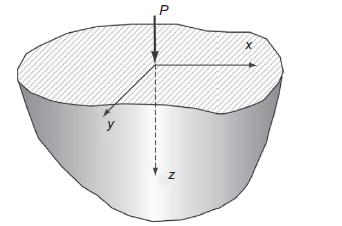
Show that Cerruti’s problem of Fig. 13.3 is solved by the Galerkin vector and Lame´’s potential specified in relations (13.3.15). Develop the expressions for the Cartesian displacements and stresses:Fig 13.3Equation 13.3.15 P R U= "=+HAR [1 + + (1-2)(~+2 (8+2F)] 4R R+z (R+z) Pxy 1 1-2v Px 12v
Both the Galerkin vector and Love’s strain function were to satisfy the biharmonic equation.If however, these representations were also harmonic, justify that the resulting stresses will all be independent Poisson’s ratio for the case of traction-only boundary conditions.
In three dimensions, often a special case of Poisson’s ratio will greatly simplify the problem solution. Show for the special case of v = 1/2, that the displacement and stress solutions for the Kelvin and Boussinesq problems simplify and that their respective results are very similar.
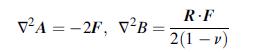
Explicitly justify that the Papkovich functions A and B satisfy relations (13.4.9).Equation 13.4.9 VA -2F, VB = R.F 2(1-v)
For the axisymmetric case, the Papkovich functions reduced to the Boussinesq potentials B and Az defined by relations (13.4.11). Show that the general forms for the displacements and stresses in cylindrical coordinates are given by:Equation 13.4.11 18 Mr = 2 r (8+ (1)), H6 = 0, Mc= 4(1-v), Or= 0 V
Using the results of Exercise 13.14, verify that the displacement and stress fields for the Boussinesq problem of Example 13.4 are given by (13.4.20) and (13.4.21). Note the interesting behavior of the radial displacement, that ur > 0 only for points where z/R > (1– 2v)R/(R + z). Show that
The displacement field for the Boussinesq problem was given by (13.4.20). For this case, construct a displacement vector distribution plot, similar to the two-dimensional case shown in Fig. 8.22. For convenience, choose the coefficient P/4πμ = 1 and take v = 0.3. Compare the two- and
Consider an elastic half-space with σz = 0 on the surface z = 0. For the axisymmetric problem, show that the Boussinesq potentials must satisfy the relation Az = 2∂B/∂z within the half-space.
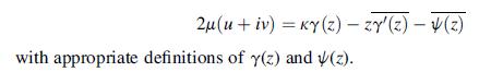
Consider the Papkovich representation for the two-dimensional plane strain case where A = A1(x,y)e1 + A2(x,y) e2 and B = B(x,y). Show that this representation will lead to the complex variable formulation: 2u(u + iv) = Ky (2) - ZY'(z) - Y(2) with appropriate definitions of y(z) and (z).
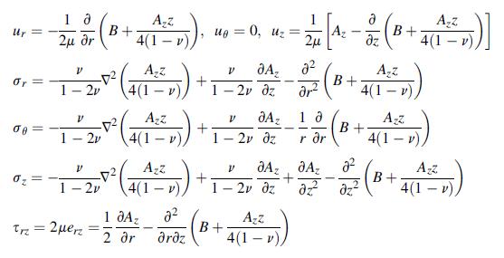
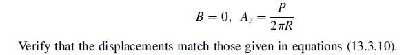
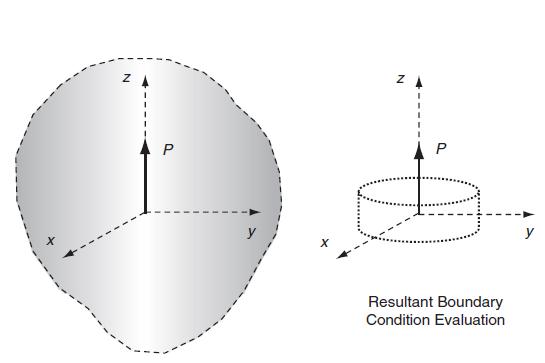
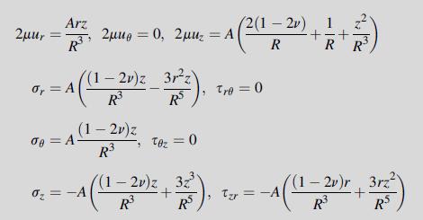
Show that Kelvin’s problem of Fig. 13.1 may be solved using the axisymmetric Papkovich functions (Boussinesq potentials):Fig 13.1Equation 13.3.10 P 2 TR Verify that the displacements match those given in equations (13.3.10). B = 0, A=
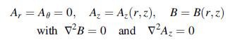
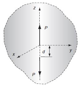
A force doublet is commonly defined as two equal but opposite forces acting in an infinite medium as shown in the following figure. Develop the stress field for this problem by superimposing the solution from Example 13.1 onto that of another single force of –P acting at the point z =–d. In
Using the results of Exercise 13.20, continue the superposition process by combining three force doublets in each of the coordinate directions. This results in a center of dilatation at the origin as shown in the figure. Using spherical coordinate components, show that the stress field for this
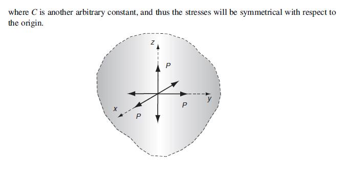
Using the basic field equations for spherical coordinates given in Appendix A, formulate the elasticity problem for the spherically symmetric case, where uR = u(R), u∅ = uθ = 0. In particular, show that the governing equilibrium equation with zero body forces becomes:Data from appendix a 2 du 2
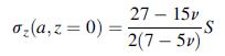
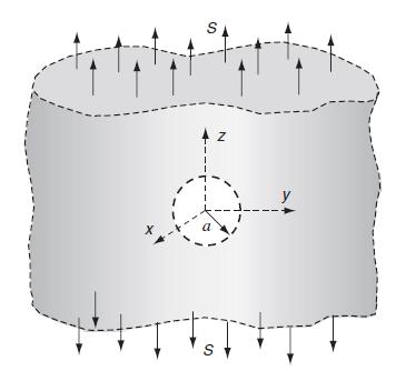
Using the results of Exercise 13.22, solve the problem of a stress-free spherical cavity in an infinite elastic medium under uniform far-field stress σ∞x =σ∞y = σ∞z = S. Explicitly show that the stress concentration factor for this case is K = 1.5 and compare this value with the
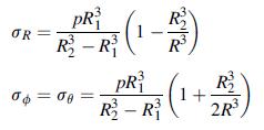
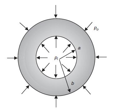
Using the results of Exercise 13.22, solve the problem of a thick-walled spherical shell with inner radius R1 loaded with uniform pressure p1, and with outer radius R2 loaded with uniform pressure p2. For the special case with p1 = p and p2 = 0, show that the stresses are given by:Data from
Using the general solution forms of Exercise 13.22, solve the problem of a rigid spherical inclusion of radius a perfectly bonded to the interior of an infinite body subjected to uniform stress at infinity of σ∞R = S. Explicitly show that the stress field is given by:Determine the nature of the
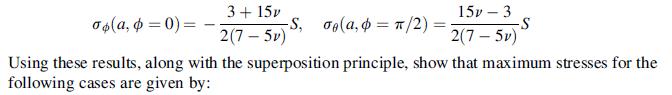
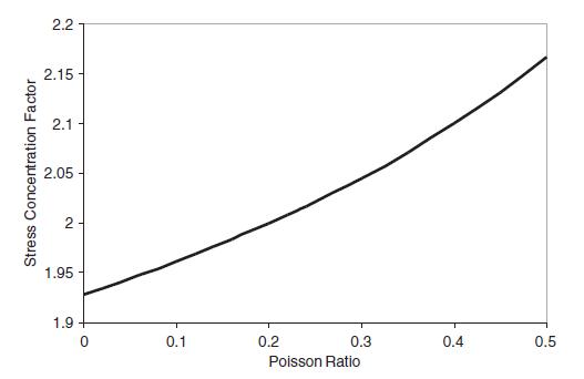
Consider the three-dimensional stress concentration problem given in Example 13.5. Recall that the maximum stresses occur on the boundary of the spherical cavity (r = a). With respect to the problem geometry shown in Fig. 13.5, the maximum stress component was found to be:Fig 13.5Other stress
Generate plots of the stress concentration factor versus Poisson’s ratio (similar to Fig. 13.6) for each case in Exercise 13.26. Compare the results.Fig 13.6Data from exercise 13.26Consider the three-dimensional stress concentration problem given in Example 13.5. Recall that the maximum stresses
There has been some interesting research dealing with materials that have negative values of Poisson’s ratio; recall from fundamental theory–1≤ v≤ 1/2. Beginning studies of this concept were done by Lakes (1987) and commonly these types of materials have specialized internal microstructures
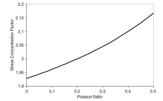
Using the Morera stress function formulation, define:where ∅ is independent of z. Show that this represents plane strain conditions with ∅ equal to the usual Airy stress function. $13 || 1 220,1, 023 || 1 224,2, P12,12= 12/4
Consider the second order stress tensor representation σij = ∅,kkδij –∅,ij, where∅is a proposed stress function. First show that this scheme gives a divergence-less stress; i.e. σij,j = 0. Next using this representation in the general compatibility equations (5.3.3) with no body forces
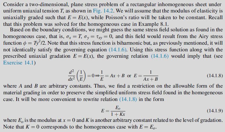
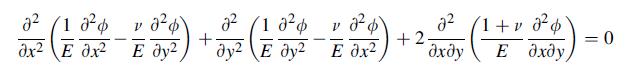
Show that, for the case of plane stress, the governing compatibility relation in terms of the Airy stress function is given by (14.1.6).Equation 14.1.6 (01 001) =0 v dy2E dy2E dx +2 2 1 + va xy E axdy, = 0 Next determine the reduced form of this equation for the special case E = E(x) and v =
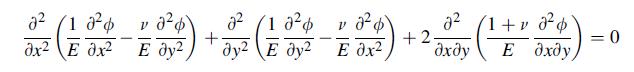
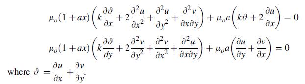
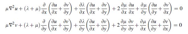
Consider a special case of Eq. (14.1.4). Parameswaran and Shukla (1999) presented a two dimensional study where the shear modulus and Lame´’s constant varied as μ(x) = μo(1 + ax) and λ(x) = kμ(x), where μo, a, and k are constants. For such a material, show that in the absence of body forces
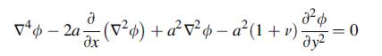
Parameswaran and Shukla (2002) recently presented a fracture mechanics study of nonhomogeneous material behavior related to functionally graded materials. They investigated a two-dimensional plane stress problem where Poisson’s ratio remained constant, but Young’s modulus varied as E(x) = $22 v - 20%+ (V) + a\ - a(1 + v); dx 0$
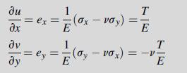
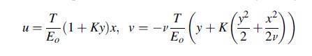
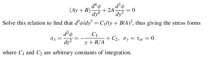
Explicitly integrate relations (14.1.10) and develop the displacements relations (14.1.11).Equation 14.1.10Equation 14.1.11 = ex :(ox way) E 1 = ly = = (dy vax) = = E T E T E
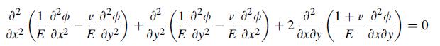
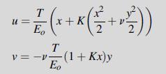
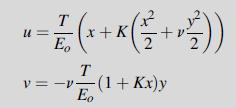
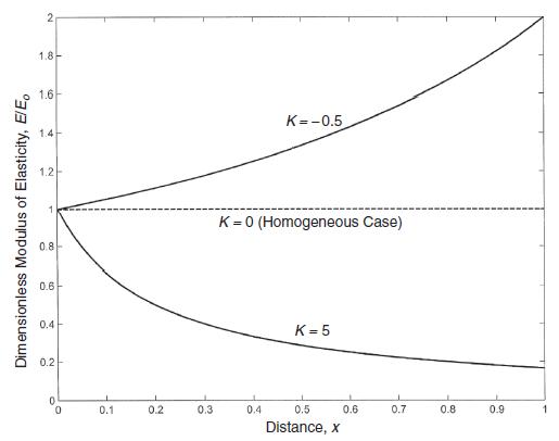
Plot horizontal and vertical displacement contours of relations (14.1.11) in the unit domain 0 ≤ (x, y) ≤ 1 for cases K=–0.5 and 5. Normalize values with respect to T/Eo and take v = 0.3. Qualitatively compare these results with those expected for the homogeneous case K = 0.Equation 14.1.11
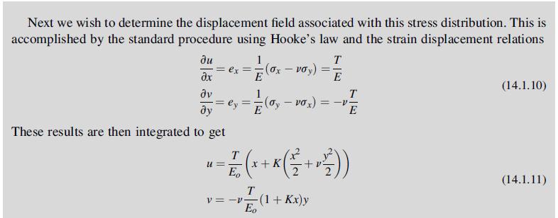
Following the scheme used in Example 14.1, consider the same stress field case ∅ = Ty2/2 but with modulus variation in the y-direction, E = E(y). First show that the required modulus variation is given by E = Eo / (1 + Ky). Next determine the resulting displacement field assuming as before zero
Consider the plane stress inhomogeneous case with only variation in elastic modulus given by E = E(y) = 1/ (Ay + B). Further assume that the Airy function depends only on y, ∅ = ∅(y). Show that governing relation (14.1.6) reduces to the ordinary differential equation:Equation 14.1.6 d b (Ay+B)-
The stress state σx = σy = 0, τ xy = T = constant corresponds to the Airy stress function ∅ =–Txy. For this case with constant Poisson’s ratio, show that the general equation (14.1.6) greatly reduces and gives the result that the allowable Young’s modulus must be of the form 1/E = f(x)
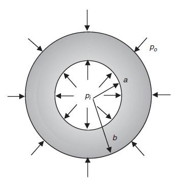
Consider a stress function formulation for the axisymmetric problem discussed in Section 14.2. The appropriate compatibility relation for this case has been previously developed in Example 8.11; see (8.4.76). Using the plane stress Hooke’s law, express this compatibility relation in terms of
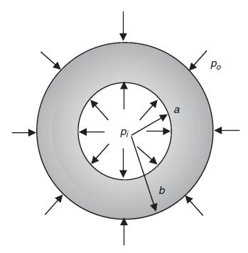
For the hollow cylinder problem shown in Fig. 14.5, use the given boundary conditions to explicitly determine the arbitrary constants A and B and the stress relations (14.2.6).Fig 14.5Equation 14.2.6 Pi b a Po
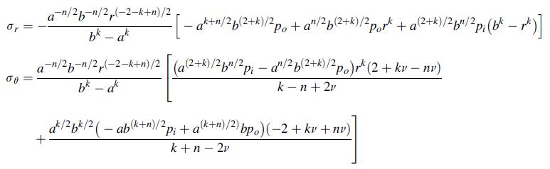
For the problem in Fig. 14.5 with only internal pressure, show that the general stress field (14.2.6) reduces to relations (14.2.7).Fig 14.5Equation 14.2.6Equation 14.2.7 Pi a od
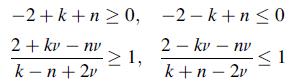
For the hollow cylinder problem illustrated in Fig. 14.5, show that the usual restrictions on Poisson’s ratio, 0 ≤ v≤ 1/2, and n > 0 imply that:Using these results, develop arguments to justify that the stresses in solution (14.2.7) must satisfy σr θ > 0 in the cylinder’s domain.
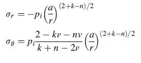
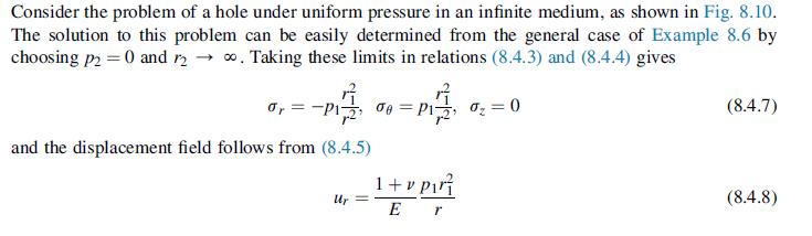
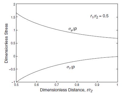
Following procedures similar to those for the homogeneous problem (see Section 8.4.1), develop the following stress field for a pressurized hole in an infinite nonhomogeneous medium with moduli variation given by (14.2.3)Plot the dimensionless stress fields for this case using the same parameters n
For the inhomogeneous rotating disk problem with v = 0, explore the solution for the special case of n = 3 and show that the stresses reduce to:Also determine the displacement solution and show the surprising result that u(0) > 0. This strange behavior has been referred to as a cavitation at the
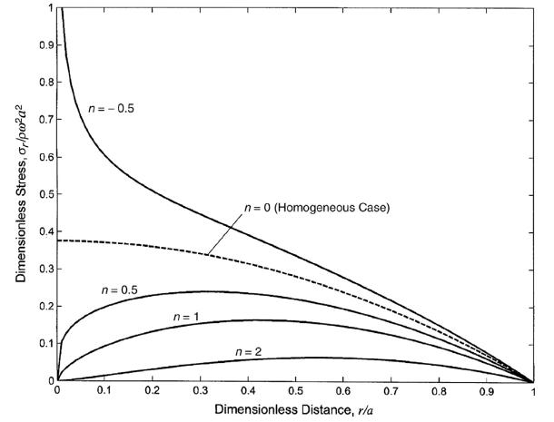
Using MATLAB or similar software, make a plot similar to Fig. 14.13 showing the behavior of the hoop stress σθ for the case with v = 0 and n =–0.5, 0, 0.5, 1, 2. Discuss your results.Fig 14.13 Dimensionless Stress, o,/poa 0.9 0.8 0.6 0.7H 0.5 0.4 0.3 0.2 F 0.1 T n=-0.5 n=0.5 0.1 0.2 n=1 0.3
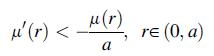
Using the design criterion (14.3.14), incorporate the fundamental equations for the inhomogeneous rotating disk problem to explicitly develop the required gradation given by relation (14.3.15).Equation 14.3.14Equation 14.3.15 or 08, re(0, a) Or
Rather than using polar coordinates to formulate the inhomogeneous half-space problem of Section 14.4, some researchers have used Cartesian coordinates instead. Using the x, z-coordinates as shown in Fig. 14.14, consider the plane strain case with inhomogeneity only in the shear modulus such that
Consider the axisymmetric half-space problem shown in Fig. 14.19 for the case where only Poisson’s ratio is allowed to vary with depth coordinate v = v(z). Using cylindrical coordinates (r, θ, z) to formulate the problem, first show that the stress field can be expressed by:Fig 14.19 r = - 2 0 =
For the antiplane strain problem, verify that transformation (14.5.5) will reduce the governing equilibrium equation to relation (14.5.6). Next show that the separation of variables scheme defined by (14.5.7) will lead to the two equations (14.5.8).Equation 14.5.5Equation 14.5.6Equation
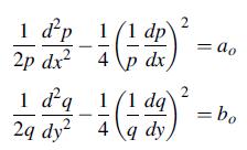
Explicitly show that the inhomogeneity functions p(x) = e–αΙxΙ and q(y) = e–βΙyΙ, that were used for the antiplane crack problem, do in fact satisfy relations (14.5.9) with ao = α2/4 and bo = β2/4.Equation 14.5.9 1 d'p 2p dx 1(1 dp 4 (14) dx 1 dq 1 1 dq 29 dy 4 dy 2 = ao 2 = bo
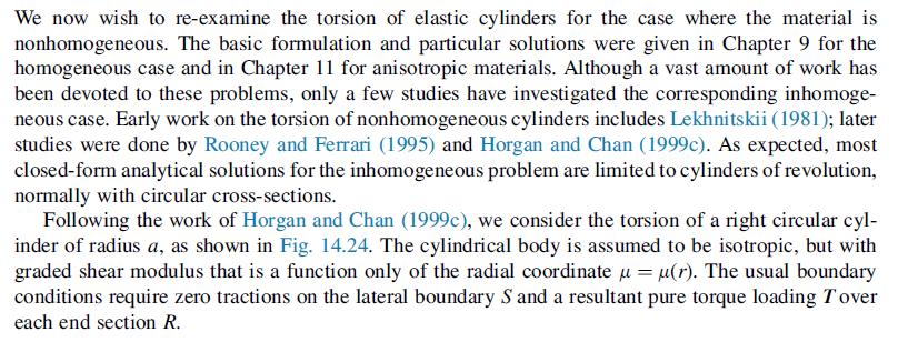
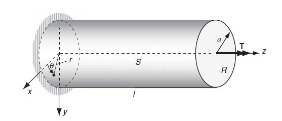
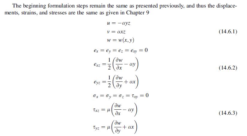
For the torsion problem discussed in Section 14.6, explicitly justify the reductions in polar coordinates summarized by relations (14.6.8) and (14.6.9).Data from section 14.6Equation 14.6.8Equation 14.6.9 We now wish to re-examine the torsion of elastic cylinders for the case where the material is
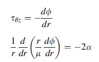
Verify that the general solutions to equations (14.6.9) are given by (14.6.11) and (14.6.12) for the torsion problem.Equation 14.6.9Equation 14.6.11Equation 14.6.12 Toz do dr 1 d (r do dr r dr = -2
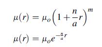
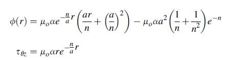
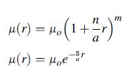
For the torsion problem, verify the solutions (14.6.14) and (14.6.15) for the gradation model (14.6.13)1.Equation 14.6.14Equation 14.6.15Equation 14.6.13 [2(a-1) + Man (-), m 3 a m = 1 (r) = 2 n | -^ a[r - () 08|1 + ] +^ - (0g|1 + r)], m log|1+n|| 1+ m = -1 n
For the torsion problem, verify the solutions (14.6.16) for the gradation model (14.6.13)2.Equation 14.6.16Equation 14.6.13 **(+)) - A (+2) - -n e n n n (r) = oder (ar Mae Toz Moare a
Investigate the issue of finding the location of (τ θz)max for the torsion problem. First verify the results given by (14.6.17) and (14.6.18). Next apply these general relations to the specific gradation models given by (14.6.13)1,2, and develop explicit results for locations of the
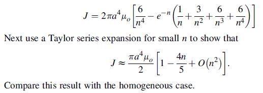
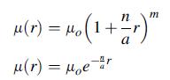
Show that the torsional rigidity for the exponential gradation case (14.6.13)2 is given by:Equation 14.6.13 6 6 J = 250 57 - " ( 2 + 3 + 2/ n4 n n n Next use a Taylor series expansion for small n to show that 4n = a m [1-45 +0 (1)]. 2 Compare this result with the homogeneous case.
Explicitly show that the fourth-order polynomial Airy stress functionwill not satisfy the biharmonic equation unless 3A40 + A22 + 3A04 = 0. A40x+ + A22xy + A04y+
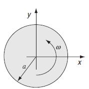
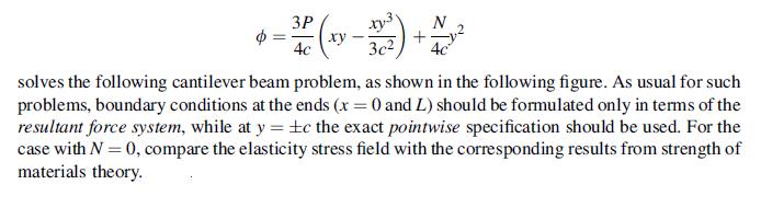
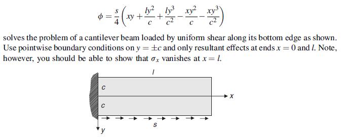
Show that the Airy function:solves the following cantilever beam problem, as shown in the following figure. As usual for such problems, boundary conditions at the ends (x = 0 and L) should be formulated only in terms of the resultant force system, while at y = ± c the exact pointwise specification
Verify that the Airy stress function: e solves the problem of a cantilever beam loaded by uniform shear along its bottom edge as shown. Use pointwise boundary conditions on y = tc and only resultant effects at ends x = 0 and 1. Note, however, you should be able to show that ox vanishes at x = l. 1
A triangular plate of narrow rectangular cross-section and uniform thickness is loaded uniformly along its top edge as shown in the following figure. Verify that the Airy stress function: p cot a -2 (1-a cota) [- tan a + xy + (x + y) (a tan-)] solves this plane problem. For the particular case of
A triangular plate of narrow rectangular cross-section and uniform thickness carries a uniformly varying loading along its top edge as shown. Verify that the Airy stress function: p=[a14 cos+b14 sin 0 + a31 cos 30 +b31 sin 30] solves this plane problem. p(x) = kx r 0 X
Explicitly determine the bending stress σx for the problem in Example 8.4. For the case l/c = 3, plot this stress distribution through the beam thickness at x = l/2, and compare with strength of materials theory. For long beams (l >> c), show that the elasticity results approach the strength of
Under the conditions of polar axis symmetric, verify that the Navier equations (5.4.4) reduce to relation (8.3.10). Refer to Example 1.5 to evaluate vector terms in (5.4.4) properly. Next show that the general solution to this CauchyeEuler differential equation is given by (8.3.11). Finally, use
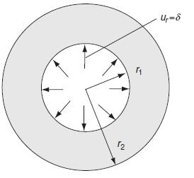
Through a shrink-fit process, a rigid solid cylinder of radius r1 +δ is to be inserted into the hollow cylinder of inner radius r1 and outer radius r2 (as shown in the following figure). This process creates a displacement boundary condition ur(r1) = δ. The outer surface of the hollow cylinder
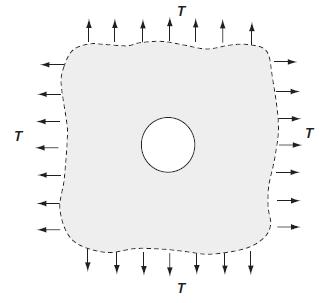
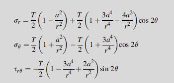
Using superposition of the stress field (8.4.15) given in Example 8.7, show that the problem of equal biaxial tension loading on a stress-free hole as shown in the figure is given by Eq. (8.4.9).Equation 8.4.15Equation 8.4.9Data from example 8.7 T T T T
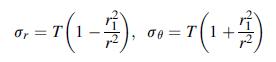
Consider the quarter plane domain problem shown in Fig. 8.17 but this time with a uniformly distributed normal loading N along the y-axis in the x-direction. Use the proposed general Airy function (8.4.19), and apply four proper boundary conditions to determine the unknown constants. Develop the
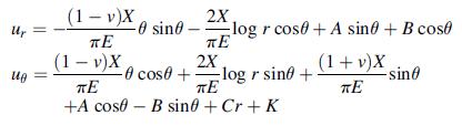
Show that plane stress displacements for the Flamant problem in Section 8.4.7 under only tangential force X are given by:Data from section 8.4.7 My (1 v) - - -0 sin (1 v)X, -0 cost + 2X, 20 log r cos + A sin + B cost log r sin + +A cost - B sino + Cr + K (1 + v)X -sina
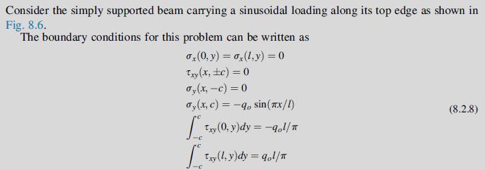
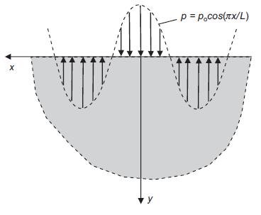
Consider an elastic half-space loaded over its entire free surface with a sinusoidal pressure as shown. Using a portion of the general solution (8.2.6), show that an Airy stress function of the form ∅ = cos βx [Be–βy + Dye–βy] will satisfy the appropriate boundary and far-field conditions
Following a similar solution procedure as used in Section 8.4.9, show that the solution for a half-space carrying a uniformly distributed shear loading t is given by: 0x = Ox 2 Txy M dy=[cos20 - cos201)] 2 [4log(sin0/sin0) - cos202 + cos20)] X t 2 [2(02-01)+sin202 - sin201] 02 a a 0
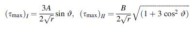
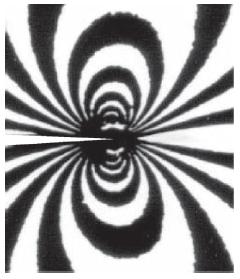
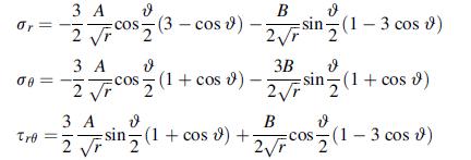
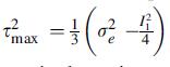
Photoelastic studies of the stress distribution around the tip of a crack have produced the isochromatic fringe pattern (opening mode I case) as shown in the figure. Using the solution given in (8.4.57), show that maximum shear stresses for each mode case are given by:Next, plot contours of
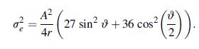
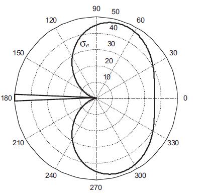
Using results from Exercises 3.19 and 8.43, show that the mode I crack tip von Mises stress is given by:Next solve this equation for the radial coordinate and make a polar plot for a typical von Mises stress contour (σe = constant) about the crack tip. Result should look like the following figure,
Show that the curved beam problem with given end loadings can be solved by super imposing the solution from the Airy function ∅ = [Ar3 + (B/r) + Cr + Dr log r] cosθ with the pure bending solution (8.4.61).Equation 8.4.61 Or = 00 4M [ab N Tre = 0 4M -1 N -log (2/2) 10 | + blog (7) + a log ab ()]
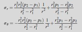
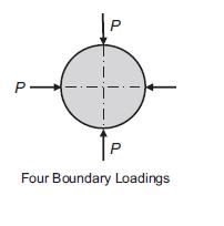
Consider an extension of Exercise 8.51 in which we wish to explore the stress distribution in a circular disk under an increasing number of boundary loadings. First show that for case:(a). With four loadings, the center stresses are given by σx = σy =–4P/πD, τ, xy = 0, where D is the disk
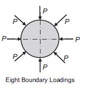
Using relation (8.5.4)1 along with Hooke’s law for plane stress, show that the surface stresses under a frictionless indenter are given by the hydrostatic state Ꝺ̅x = Ꝺ̅y = – p(x). This situation would tend to restrict the surface layer to deform plastically under such loading.Equation

Showing 400 - 500 of 709

1
2
3
4
5
6
7
8

Step by Step Answers

Services

Sitemap
Fun
Definitions
Become Tutor
Used Textbooks
Study Help Categories
Recent Questions
Expert Questions
Campus Wear
Sell Your Books

Company Info

Security
Copyrights
Privacy Policy
Terms & Conditions
SolutionInn Fee
Scholarship
Online Quiz
Give Feedback, Get Rewards

Get In Touch

About Us
Contact Us
Career
Jobs
FAQ
Student Discount
Campus Ambassador

Secure Payment

Download Our App

© 2026 SolutionInn. All Rights Reserved