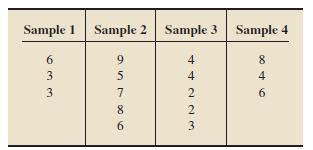
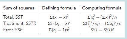
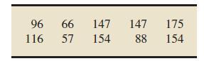
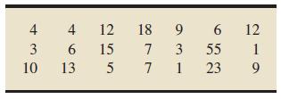
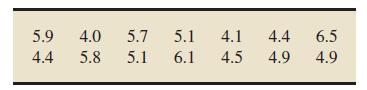
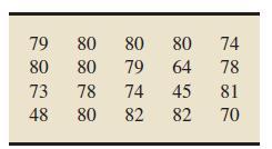
All Matches
Solution Library
Expert Answer
Textbooks
Search Textbook questions, tutors and Books
Oops, something went wrong!
Change your search query and then try again
Toggle navigation
FREE Trial
S
Books
FREE
Tutors
Study Help
Expert Questions
Accounting
General Management
Mathematics
Finance
Organizational Behaviour
Law
Physics
Operating System
Management Leadership
Sociology
Programming
Marketing
Database
Computer Network
Economics
Textbooks Solutions
Accounting
Managerial Accounting
Management Leadership
Cost Accounting
Statistics
Business Law
Corporate Finance
Finance
Economics
Auditing
Ask a Question
Search
Search
Sign In
Register
study help
statistics
elementary statistics a step by step approach
Questions and Answers of
Elementary Statistics A Step By Step Approach
Exercise contain graphs portraying the decision criterion for a one-mean z-test. The curve in each graph is the normal curve for the test statistic under the assumption that the null hypothesis is
Determine the critical value(s) for a one-mean z-test. For each exercise, draw a graph that illustrates your answer. A two-tailed test with α = 0.05.
Exercise contain graphs portraying the decision criterion for a one-mean z-test. The curve in each graph is the normal curve for the test statistic under the assumption that the null hypothesis is
Determine the critical value(s) for a one-mean z-test. For each exercise, draw a graph that illustrates your answer.A right-tailed test with α = 0.05.
Determine the critical value(s) for a one-mean z-test. For each exercise, draw a graph that illustrates your answer. A left-tailed test with α = 0.01.
Determine the critical value(s) for a one-mean z-test. For each exercise, draw a graph that illustrates your answer. A left-tailed test with α = 0.05.
Determine the critical value(s) for a one-mean z-test. For each exercise, draw a graph that illustrates your answer. A right-tailed test with α = 0.01
In each Exercise, we have given the P-value for a hypothesis test. For each exercise, refer to Table 9.8 to determine the strength of the evidence against the null hypothesis.P = 0.027P = 0.184 TABLE
In each Exercise, we have given the P-value for a hypothesis test. For each exercise, refer to Table 9.8 to determine the strength of the evidence against the null hypothesis.P = 0.184 TABLE
In each Exercise, we have given the P-value for a hypothesis test. For each exercise, refer to Table 9.8 to determine the strength of the evidence against the null hypothesis.P = 0.004 TABLE
In each Exercise, we have given the P-value for a hypothesis test. For each exercise, refer to Table 9.8 to determine the strength of the evidence against the null hypothesis.P = 0.086 TABLE
In each Exercise, we have given the P-value for a hypothesis test. For each exercise, refer to Table 9.8 to determine the strength of the evidence against the null hypothesis.P = 0.012 TABLE
We have given the value obtained for the test statistic, z, in a one-mean z-test. We have also specified whether the test is two-tailed, left-tailed, or right-tailed. Determine the P-value in each
We have provided a sample mean, sample size, and population standard deviation. In each case, use the one-mean z-test to perform the required hypothesis test at the 5% significance level.x̄ = 21, n
We have provided a sample mean, sample size, and population standard deviation. In each case, use the one-mean z-test to perform the required hypothesis test at the 5% significance level.x̄ = 24, n
We have provided a sample mean, sample size, and population standard deviation. In each case, use the one-mean z-test to perform the required hypothesis test at the 5% significance level.x̄ = 23, n
We have provided a sample mean, sample size, and population standard deviation. In each case, use the one-mean z-test to perform the required hypothesis test at the 5% significance level.x̄ = 20, n
Suppose that you want to perform a hypothesis test for a population mean based on a small sample but that preliminary data analyses indicate either the presence of outliers or that the variable under
Pertain to P-values for a one-mean t-test. For each exercise, do the following tasks.a. Use Table IV in Appendix A to estimate the P-value.b. Based on your estimate in part (a), state at which
In each of Exercise, we have provided a sample mean, sample standard deviation, and sample size. In each case, use the one-mean t-test to perform the required hypothesis test at the 5% significance
Provides a type of sampling (independent or paired), sample size(s), and a figure showing the results of preliminary analyses on the sample(s). For independent samples, the graphs are for the two
In each of Exercise, we have presented a confidence interval (CI) for the difference, μ1 − μ2, between two population means. Interpret each confidence interval.95% CI is from −20 to −15.
In each of Exercise, we have presented a confidence interval (CI) for the difference, μ1 − μ2, between two population means. Interpret each confidence interval.90% CI is from −10 to −5.
In each of Exercise, we have presented a confidence interval (CI) for the difference, μ1 − μ2, between two population means. Interpret each confidence interval.90% CI is from 5 to 10.
Provides a type of sampling (independent or paired), sample size(s), and a figure showing the results of preliminary analyses on the sample(s). For independent samples, the graphs are for the two
In each of Exercise, we have presented a confidence interval (CI) for the difference, μ1 − μ2, between two population means. Interpret each confidence interval.99% CI is from −20 to 15.
Provides a type of sampling (independent or paired), sample size(s), and a figure showing the results of preliminary analyses on the sample(s). For independent samples, the graphs are for the two
Suppose, in Example 10.2, you want to decide whether the mean salary of faculty in private institutions is greater than the mean salary of faculty in public institutions. State the null and
Hypothesis tests are proposed. For each hypothesis test,a. identify the variable.b. identify the two populations.c. determine the null and alternative hypotheses.d. classify the hypothesis test as
Repeat parts (b)–(e) of Exercise 11.9 for samples of size 3.(b)–(e) of Exercise 11.9b. The first column of the following table provides the possible samples of size 2, where each person is
E. Bergman et al. conducted a study to determine, among other things, the impact that scheduling recess before or after the lunch period has on wasted food fo students in a grades three through five.
We have provided summary statistics for independent simple random samples from two populations. Preliminary data analyses indicate that the variable under consideration is normally distributed on
Explain why sp is called the pooled sample standard deviation.
We have provided summary statistics for independent simple random samples from two populations. Preliminary data analyses indicate that the variable under consideration is normally distributed on
Phyllodes tumors of the breast are rare tumors that represent less than one percent of growths in the breast. Researchers I. Youn et al. presented characteristics of phyllodes tumors in the article
An intervention program designed by the Stockholm Transit District was implemented to improve the work conditions of the city’s bus drivers. Improvements were evaluated by G. Evans et al., who
L. Gross back et al. examined mandate perceptions and their causes in the paper “Comparing Competing Theories on the Causes of Mandate Perceptions”. Following are data on the percentage of
The null hypothesis is H0:μ1 = μ2 and the alternative hypothesis is as specified. We have provided data from a simple random paired sample from the two populations under consideration. In each
The null hypothesis is H0: μ1 = μ2 and the alternative hypothesis is as specified. We have provided data from a simple random paired sample from the two populations under consideration. In each
The null hypothesis is H0 :μ1 = μ2 and the alternative hypothesis is as specified. We have provided data from a simple random paired sample from the two populations under consideration. In
The null hypothesis is H0: μ1 = μ2 and the alternative hypothesis is as specified. We have provided data from a simple random paired sample from the two populations under consideration. In each
Cooling down with a cold drink before exercising in the heat is believed to help an athlete perform. Researcher J. Dugas explored the difference between cooling down with an ice slurry (slushy) and
Apply Procedure 10.6 on to obtain the required confidence interval. Interpret your result in each case.Refer to Exercise 10.123a. Determine a 95% confidence interval for the difference between the
Refer to Exercise 10.128 and find a 98% confidence interval for the difference between the mean times to fatigue on a treadmill in a hot and humid environment after cooling down with cold water and
In the online paper “A Comparison of Two Computer Fonts: Serif versus Ornate Sans Serif”, researchers S. Morrison and J. Noyes studied whether the type of font used in a document affects reading
Tests. With the advent of high-speed computing, new procedures have been developed that permit statistical inferences to be performed under less restrictive conditions than those of classical
We have given the number of successes and the sample size for a simple random sample from a population. In each case, do the following.a. Determine the sample proportion.b. Decide whether using the
Use either the critical-value approach or he P-value approach to perform the required hypothesis test.In the United States, approximately 450,000 vasectomies are performed each year. In this surgical
We have given the numbers of successes and the sample sizes for simple random samples for independent random samples from two populations. In each case,a. Use the two-proportions plus-four z-interval
For a χ2-curve with df = 10, determinea. χ20.05. b. χ20.025.
For a χ2-curve with df = 10, determinea. χ20.05. b. χ20.01.
We have given the relative frequencies for the null hypothesis of a chi-square goodness-of-fit test and the sample size. In each case, decide whether Assumptions 1 and 2 for using that test are
We have provided distribution and the observed frequencies of the values of a variable from a simple random sample of a population. In each case, use the chi-square goodness-of-fit test to decide, at
The Higher Education Research Institute of the University of California, Los Angeles, publishes information on the characteristics of incoming college freshmen in The American Freshman. In 2000,
Refer to Table 12.11. Consider the variables “gender” and “college.”a. Group the bivariate data for these two variables into a contingency table.b. Determine the conditional distribution of
Consider the variables “class level” and “college.”a. Group the bivariate data for these two variables into a contingency table.b. Determine the conditional distribution of class level within
The U.S. Census Bureau publishes information about housing units in American Housing Survey for the United States. The following table cross-classifies single-unitFor single-unit occupied housing
We have given the number of possible values for two variables of a population. For each exercise, determine the maximum number of expected frequencies that can be less than 5 in order that Assumption
Fill in the blank: If a variable has only two possible values, the chi-square homogeneity test provides a procedure for comparing several ___________ populations.
A chi-square homogeneity test is to be conducted to decide whether a difference exists among the distributions of a variable of six populations. The variable has five possible values. What are the
In Exercises,a. Obtain and interpret the quartiles.b. Determine and interpret the interquartile range.c. Find and interpret the five-number summary.d. Identify potential outliers, if any.e. Construct
The National Association of Colleges and Employers (NACE) conducts surveys of salary offers to new college graduates and publishes the results in Salary Survey. The following diagram provides
In the Exercise, we give linear equations. For each equation,a. Find the y-intercept and slope.b. Determine whether the line slopes upward, slopes downward, or is horizontal, without graphing the
In each of Problems 9–11, fill in the blank.The line that best fits a set of data points according to the least squares criterion is called the_________line.
In the Exercise, we give linear equations. For each equation,a. Find the y-intercept and slope.b. Determine whether the line slopes upward, slopes downward, or is horizontal, without graphing the
In the Exercise, we identify the y-intercepts and slopes, respectively, of lines. For each line,a. Determine whether it slopes upward, slopes downward, or is horizontal, without graphing the
In Exercises,a. Obtain and interpret the quartiles.b. Determine and interpret the interquartile range.c. Find and interpret the five-number summary.d. Identify potential outliers, if any.e. Construct
Researchers in obesity wanted to compare the effectiveness of dieting with exercise against dieting without exercise. Seventy-three patients were randomly divided into two groups. Group 1, composed
Consider the following three data sets.a. Assuming that each of these data sets is sample data, compute the standard deviations. (Round your final answers to two
A study published by E. Anion et al. in the British Medical Journal (Vol. 282, pp. 283–286) examined the steady-state hemoglobin levels of patients with three different types of sickle cell
In each of Exercise,a. Use the technology of your choice to obtain boxplots for the data sets, using the same scale.b. Compare the data sets by using your results from part (a), paying special
In each Exercise,a. Use the technology of your choice to obtain boxplots for the data sets, using the same scale.b. Compare the data sets by using your results from part (a), paying special attention
In Section 3.2, we analyzed the heights of the starting five players on each of two men’s college basketball teams. The heights, in inches, of the players on Team II are 67, 72, 76, 76, and 84.
In Exercise, we have provided simple data sets for you to practice the basics of finding a.a. Population mean.b. Population standard deviation.3, 5, 7
Showing 400 - 500
of 1607
1
2
3
4
5
6
7
8
9
10
11
12
13
14
15
Last