New Semester Started Get 50% OFF Study Help! --h --m --s Claim Now

Question Answers

Textbooks

Find textbooks, questions and answers

Oops, something went wrong!

Change your search query and then try again

Result Not Found

Books FREE
Study Help
Tutors
AI Study Planner NEW
Sell Books

Search
Sign In
Register

study help
statistics
elementary statistics a step by step approach

Elementary Statistics 9th Edition Neil A Weiss - Solutions

A value of r close to ________ indicates that there is either no linear relationship between the variables or a weak one.
A value of r close to __________indicates that the regression equation is extremely useful for making predictions.
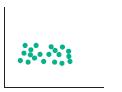
In Exercise, determine whether r is positive, negative, or zero.
A value of r close to 0 indicates that the regression equation is either useless or_________ for making predictions.
If y tends to increase linearly as x increases, the variables are ________linearly correlated.
If y tends to decrease linearly as x increases, the variables are __________ linearly correlated.
If there is no linear relationship between x and y, the variables are linearly_________.
A value of r close to −1 suggests a strong______________ linear relationship between the variables.
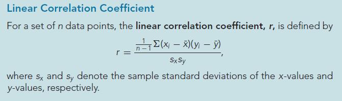
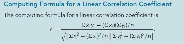
In Exercise, For each exercise, determine the linear correlation coefficient by usinga. Definition 4.8 b. Formula 4.3 Compare your answers in parts (a) and (b). Linear Correlation Coefficient For a set of n data points, the linear correlation coefficient, r, is defined by ¹₁ Σ(x₁ -
In Exercise, we repeat data from exercise. For each exercise, determine the linear correlation coefficient by usinga. Definition 4.8 b. Formula 4.3 Compare your answers in parts (a) and (b). Linear Correlation Coefficient For a set of n data points, the linear correlation coefficient, r,
In Exercise, we repeat data from exercise. For each exercise, determine the linear correlation coefficient by usinga. Definition 4.8 b. Formula 4.3 Compare your answers in parts (a) and (b). Linear Correlation Coefficient For a set of n data points, the linear correlation coefficient, r,
In Exercise, For each exercise, determine the linear correlation coefficient by usinga. Definition 4.8 b. Formula 4.3 Compare your answers in parts (a) and (b). Linear Correlation Coefficient For a set of n data points, the linear correlation coefficient, r, is defined by ¹₁ Σ(x₁ -
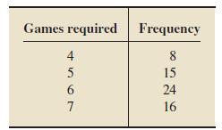
The NBA Finals of basketball is played in a best-of-seven series. The number of games necessary to decide a winner can range from four to seven. Wikipedia lists the NBA Finals winners and number of games played per series. The following table provides the number of series that were decided in 4, 5,
Determine 0!, 3!, 4!, and 7!.
This problem requires that you first obtain the gender and handedness of each student in your class. Subsequently, determine the probability that a randomly selected student in your class isa. Female.b. Left-handed.c. Female and left-handed.d. Neither female nor left-handed.
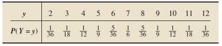
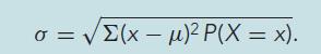
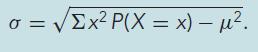
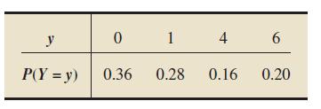
The random variable Y is the sum of the dice when two balanced dice are rolled. Its probability distribution is as follows.For each exercise, do the following tasks.a. Find and interpret the mean of the random variable.b. Obtain the standard deviation of the random variable by using one of the
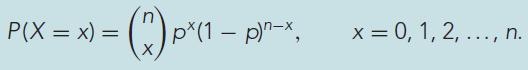
What is the binomial distribution?
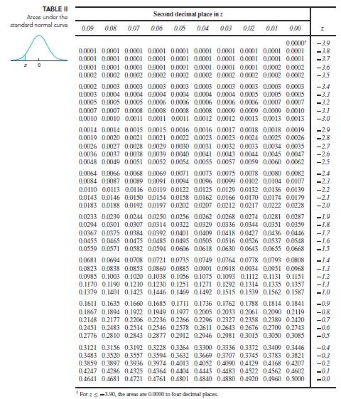
In Exercise, use Table II to obtain the required z-scores. Illustrate your work with graphs. 6.71 Obtain the z-score for which the area under the standard normal curve to its left is 0.025.Obtain the z-score for which the area under the standard normal curve to its left is 0.025.Table II TABLE
Sketch the normal distribution witha. μ = 3 and σ = 3. b. μ = 1 and σ = 3.c. μ = 3 and σ = 1.
Sketch the normal distribution witha. μ = −2 and σ = 2. b. μ = −2 and σ = 1/2.c. μ = 0 and σ = 2.
Use Table II to obtain the areas under the standard normal curve required in Exercise. Sketch a standard normal curve and shade the area of interest in each problem.Determine the area under the standard normal curve that lies to the left ofa. 2.24. b. −1.56. c. 0. d. −4.
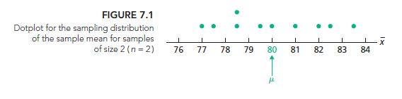
We have given population data for a variable. For each exercise, do the following tasks.a. Find the mean, μ, of the variable.b. For each of the possible sample sizes, construct a table similar to Table 7.2 and draw a dotdot plot the sampling distribution of the sample mean similar to Fig. 7.1.c.
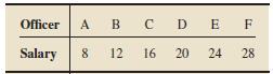
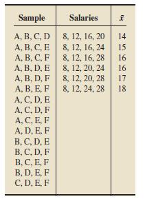
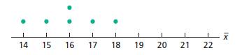
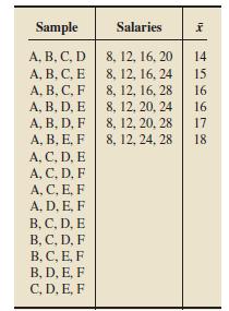
The following table gives the monthly salaries (in $1000s) of the six officers of a company.a. Calculate the population mean monthly salary, μ.There are 15 possible samples of size 4 from the population of six officers. They are listed in the first column of the following table.b. Complete the
We have given population data for a variable. For each exercise, do the following tasks.a. Find the mean, μ, of the variable.b. For each of the possible sample sizes, construct a table similar to Table 7.2 and draw a dotdot plotr the sampling distribution of the sample mean similar to Fig. 7.1.c.
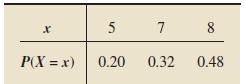
For each exercise, do the following tasks.a. Find the mean of the random variable.b. Obtain the standard deviation of the random variable by using one of the formulas given in Definition 5.10. 5 P(X=x) 0.20 X S 7 8 0.32 0.48
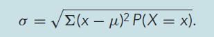
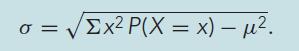
For each exercise, do the following tasks.a. Find the mean of the random variable.b. Obtain the standard deviation of the random variable by using one of the formulas given in Definition 5.10.Definition 5.10The standard deviation of a discrete random variable X is denoted σX or, when no confusion
Regarding the equal-likelihood modela. What is it?b. How are probabilities computed?
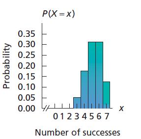
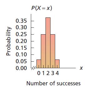
For each of the following probability histograms of binomial distributions, specify whether the success probability is less than, equal to, or greater than 0.5. Explain your answers.(a)(b) Probability 0.35 0.30 0.25 0.20 0.15 0.10 0.05 0.00 P(X=X) 1 X 01234567 Number of successes
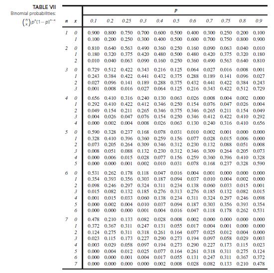
We have provided the number of trials and success probability for Bernoulli trials. Let X denote the total number of successes. Determine the required probabilities by using a. The binomial probability formula, Formula 5.4. Round your probability answers to three places.b. Table VII in
We have provided the number of trials and success probability for Bernoulli trials. Let X denote the total number of successes. Determine the required probabilities by using a. The binomial probability formula, Formula 5.4. Round your probability answers to three places.b. Table VII in
we have provided the number of trials and success probability for Bernoulli trials. Let X denote the total number of successes. Determine the required probabilities by using a. The binomial probability formula, Formula 5.4. Round your probability answers to three places.b. Table VII in
Compute 3!, 7!, 8!, and 9!.
Find 1!, 2!, 4!, and 6!.
In Exercise, use Table II to obtain the required z-scores. Illustrate your work with graphs. 6.71 Obtain the z-score for which the area under the standard normal curve to its left is 0.025.Obtain the z-score that has area 0.70 to its right.Table II TABLE II Areas under the standard normal
In Exercise, use Table II to obtain the required z-scores. Illustrate your work with graphs. 6.71 Obtain the z-score for which the area under the standard normal curve to its left is 0.025.Determine z0.33.Table II TABLE II Areas under the standard normal curve A 0.09 0.08 0.07 Second decimal place
In Exercise, use Table II to obtain the required z-scores. Illustrate your work with graphs. 6.71 Obtain the z-score for which the area under the standard normal curve to its left is 0.025.Determine z0.33.Table II TABLE II Areas under the standard normal curve A 0.09 0.08 0.07 Second decimal place
In Exercise, use Table II to obtain the required z-scores. Illustrate your work with graphs. 6.71 Obtain the z-score for which the area under the standard normal curve to its left is 0.025.Determine z0.015.Table II TABLE II Areas under the standard normal curve A 0.09 0.08 0.07 Second decimal place
In Exercise, use Table II to obtain the required z-scores. Illustrate your work with graphs. 6.71 Obtain the z-score for which the area under the standard normal curve to its left is 0.025.Find the following z-scores.a. z0.03 b. z0.005Table II TABLE II Areas under the standard normal
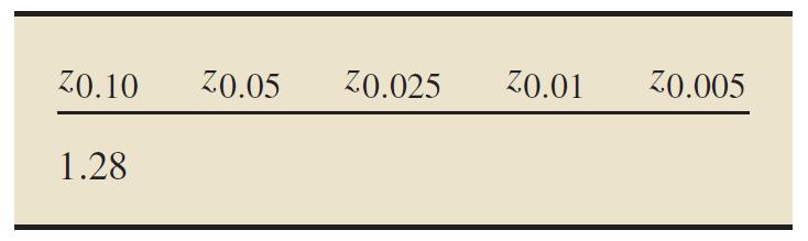
Complete the following table. 20.10 20.05 1.28 70.025 20.01 70.005
In Exercise, use Table II to obtain the required z-scores. Illustrate your work with graphs. 6.71 Obtain the z-score for which the area under the standard normal curve to its left is 0.025.Obtain the following z-scores.a. z0.20 b. z0.06Table II TABLE II Areas under the standard normal
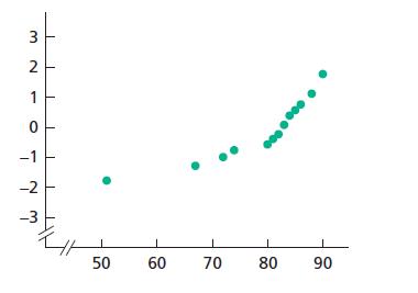
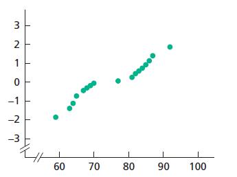
We have provided a normal probability plot of data from a sample of a population. In each case, assess the normality of the variable under consideration. 3 2 1 ŵ ↓ L 50 T 60 70 80 ******* 90
We have provided a normal probability plot of data from a sample of a population. In each case, assess the normality of the variable under consideration. 3 2 1 0 -1 -2 T 60 ******* I 70 80 90 100
Define sampling error.
We have given population data for a variable. For each exercise, do the following tasks.a. Find the mean, μ, of the variable.b. For each of the possible sample sizes, construct a table similar to Table 7.2 and draw a dotdot plotr the sampling distribution of the sample mean similar to Fig. 7.1.c.
What is the sampling distribution of a statistic? Why is it important?
We have given population data for a variable. For each exercise, do the following tasks.a. Find the mean, μ, of the variable.b. For each of the possible sample sizes, construct a table similar to Table 7.2 and draw a dotdot plotr the sampling distribution of the sample mean similar to Fig. 7.1.c.
Refer to Problem 5.a. Use the answer you obtained in Problem 5(b) and Definition 3.11 to find the mean of the variable x. Interpret your answer.b. Can you obtain the mean of the variable x̅ without doing the calculation in part (a)? Explain your answer.Problem 5(b)Complete the second and third
We have given population data for a variable. For each exercise, do the following tasks.a. Find the mean, μ, of the variable.b. For each of the possible sample sizes, construct a table similar to Table 7.2 and draw a dotdot plotr the sampling distribution of the sample mean similar to Fig. 7.1.c.
We have given population data for a variable. For each exercise, do the following tasks.a. Find the mean, μ, of the variable.b. For each of the possible sample sizes, construct a table similar to Table 7.2 and draw a dot-dot plot the sampling distribution of the sample mean similar to Fig. 7.1.c.
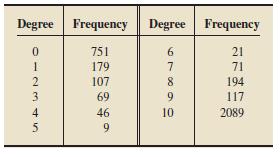
In the paper “Cloudiness: Note on a Novel Case of Frequency” Poland, during the decade. The frequency distribution of the data is presented in the following table. From the table, we find that the mean degree of cloudiness is 6.83 with a standard deviation of 4.28. Degree Frequency Degree
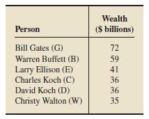
Repeat parts (b)–(e) of Exercise 7.17 for samples of size 3. Exercise 7.17Each year, Forbes magazine publishes a list of the richest people in the United States. As of September 16, 2013, the six richest Americans and their wealth (to the nearest billion dollars) are as shown in the
Repeat parts (b)–(e) of Exercise 7.17 for samples of size 1.Exercise 7.17Each year, Forbes magazine publishes a list of the richest people in the United States. As of September 16, 2013, the six richest Americans and their wealth (to the nearest billion dollars) are as shown in the following
Repeat parts (b)–(e) of Exercise 7.17 for samples of size 5.Exercise 7.17Each year, Forbes magazine publishes a list of the richest people in the United States. As of September 16, 2013, the six richest Americans and their wealth (to the nearest billion dollars) are as shown in the following
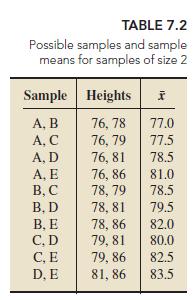
Repeat parts (b)–(e) of Exercise 7.11 for samples of size 3.Exercise 7.11a. For samples of size 2, construct a table similar to Table 7.2 on page 293. Use the letter in parentheses after each player’s name to represent each player.b. Draw a dotplot for the sampling distribution of the sample
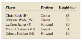
Repeat parts (b) and (c) of Exercise 7.41 for samples of size 3. For part (b), use your answer to Exercise 7.13(b).Exercise 7.41The winner of the 2012–2013 National Basketball Association (NBA) championship was the Miami Heat. One possible starting lineup for that team is as follows.a. Consider
Repeat parts (b)–(e) of Exercise 7.11 for samples of size 4.Exercise 7.11a. For samples of size 2, construct a table similar to Table 7.2. Use the letter in parentheses after each player’s name to represent each player.b. Draw a dotplot for the sampling distribution of the sample mean for
Repeat parts (b)–(e) of Exercise 7.17 for samples of size 4. Exercise 7.17Each year, Forbes magazine publishes a list of the richest people in the United States. As of September 16, 2013, the six richest Americans and their wealth (to the nearest billion dollars) are as shown in the
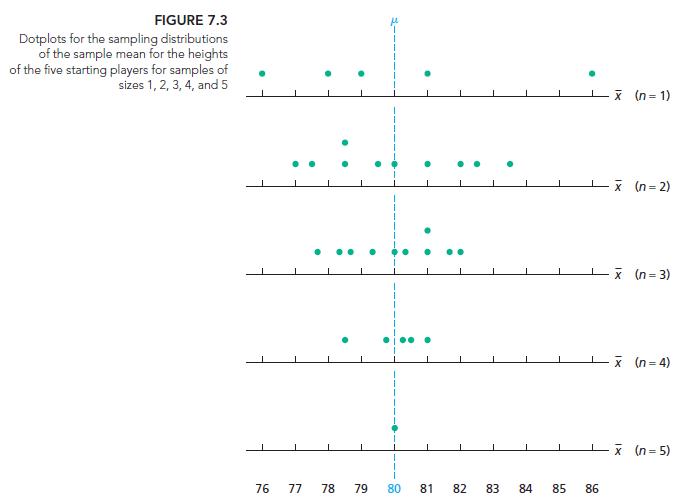
Repeat parts (b)–(e) of Exercise 7.11 for samples of size 5.Exercise 7.11a. Find the population mean height of the five players.b. For samples of size 2, construct a table similar to Table 7.2. Use the letter in parentheses after each player’s name to represent each player.c. Draw a dotplot for
The Athletic Coping Skills Inventory (ACSI) is a test to measure psychological skills believed to influence athletic performance. Researchers E. Estanol et al. studied the relationship between ACSI scores and eating disorders in dancers in the article “Mental Skills as Protective Attributes
Repeat parts (b) and (c) of Exercise 7.41 for samples of size 4. For part (b), use your answer to Exercise 7.14(b).Exercise 7.41The winner of the 2012–2013 National Basketball Association (NBA) championship was the Miami Heat. One possible starting lineup for that team is as follows.a. Consider
Repeat parts (b) and (c) of Exercise 7.41 for samples of size 5.Exercise 7.41The winner of the 2012–2013 National Basketball Association (NBA) championship was the Miami Heat. One possible starting lineup for that team is as follows.a. Determine the population mean height, μ, of the five
Assume that the variable under consideration has a density curve. Note that the answers required here may be only approximately correct.The percentage of all possible observations of a variable that lies between ____and ___ equals the area under its density curve between and is expressed as a
We have provided distribution and the observed frequencies of the values of a variable from a simple random sample of a population. In each case, use the chi-square goodness-of-fit test to decide, at the specified significance level, whether the distribution of the variable differs from the given
We have provided distribution and the observed frequencies of the values of a variable from a simple random sample of a population. In each case, use the chi-square goodness-of-fit test to decide, at the specified significance level, whether the distribution of the variable differs from the given
We have given the numbers of successes and the sample sizes for simple random samples for independent random samples from two populations. In each case,a. Use the two-proportions plus-four z-interval procedure to find the required confidence interval for the difference between the two population
We have given the numbers of successes and the sample sizes for simple random samples for independent random samples from two populations. In each case,a. use the two-proportions plus-four z-interval procedure to find the required confidence interval for the difference between the two population
Use the one-proportion plus-four z-interval procedure to find the required confidence interval. Interpret your results.A poll by Gallup asked, “If you won 10 million dollars in the lottery, would you continue to work or stop working?” Of the 1039 American adults surveyed, 707 said that they
We have given the number of successes and the sample size for a simple random sample from a population. In each case,a. use the one-proportion plus-four z-interval procedure to find the required confidence interval.b. compare your result with the corresponding confidence interval found.x = 8, n =
We have specified a margin of error, a confidence level, and a likely range for the observed value of the sample proportion. For each exercise, obtain a sample size that will ensure a margin of error of at most the one specified (provided of course that the observed value of the sample proportion
We have given the number of successes and the sample size for a simple random sample from a population. In each case, do the following tasks.a. Determine the sample proportion.b. Decide whether using the one-proportion z-interval procedure is appropriate.c. If appropriate, use the one-proportion
We have given a likely range for the observed value of a sample proportion P̂.a. Based on the given range, identify the educated guess that should be used for the observed value of P̂ to calculate the required sample size for a prescribed confidence level and margin of error.b. Identify the
We have given a likely range for the observed value of a sample proportion P̂.a. Based on the given range, identify the educated guess that should be used for the observed value of P̂ to calculate the required sample size for a prescribed confidence level and margin of error.b. Identify the
We have given a likely range for the observed value of a sample proportion P̂.a. Based on the given range, identify the educated guess that should be used for the observed value of P̂ to calculate the required sample size for a prescribed confidence level and margin of error.b. Identify the
We have given a likely range for the observed value of a sample proportion P̂.a. Based on the given range, identify the educated guess that should be used for the observed value of P̂ to calculate the required sample size for a prescribed confidence level and margin of error.b. Identify the
Refer to Problem 13. a. Find a 99% confidence interval for the difference, p1 − p2, between the proportions of men and women smartphone owners.b. Interpret your answer in part (a) in terms of the difference in percentages of men and women smartphone ownersProblem 13The Pew Internet &
In each of Exercise, assume that the population standard deviation is known and decide whether use of the z-interval procedure to obtain a confidence interval for the population mean is reasonable.The sample data contain no outliers, the sample size is 250, and the variable under consideration is
Suppose that you are considering a hypothesis test for a population mean, μ. In each part, express the alternative hypothesis symbolically and identify the hypothesis test as two tailed, left tailed, or right tailed.a. You want to decide whether the population mean is different from a specified
In each of Exercise, define the term given. Test statistic
We provide a sample mean, sample size, population standard deviation, and confidence level. In each case, perform the following tasks:a. Use the one-mean z-interval procedure to find a confidence interval for the mean of the population from which the sample was drawn.b. Obtain the margin of error
In each of Exercise, define the term given. non rejection region
In each of Exercise, define the term given.Critical values
We provide a sample mean, sample size, population standard deviation, and confidence level. In each case, perform the following tasks:a. Use the one-mean z-interval procedure to find a confidence interval for the mean of the population from which the sample was drawn.b. Obtain the margin of error
In each of Exercise, assume that the population standard deviation is known and decide whether use of the z-interval procedure to obtain a confidence interval for the population mean is reasonable.Explain your answers.The sample data contain outliers, and the sample size is 20.
In each of Exercise, assume that the population standard deviation is known and decide whether use of the z-interval procedure to obtain a confidence interval for the population mean is reasonable.The sample data contain no outliers, the variable under consideration is roughly normally distributed,
We provide a sample mean, sample size, population standard deviation, and confidence level. In each case, perform the following tasks:a. Use the one-mean z-interval procedure to find a confidence interval for the mean of the population from which the sample was drawn.b. Obtain the margin of error
In each of Exercise, assume that the population standard deviation is known and decide whether use of the z-interval procedure to obtain a confidence interval for the population mean is reasonable.The distribution of the variable under consideration is highly skewed, and the sample size is 20.
We provide a sample mean, sample size, population standard deviation, and confidence level. In each case, perform the following tasks:a. Use the one-mean z-interval procedure to find a confidence interval for the mean of the population from which the sample was drawn.b. Obtain the margin of error
Explain the effect on the margin of error and hence the effect on the accuracy of estimating a population mean by a sample mean.Increasing the sample size while keeping the same confidence level
A. Ehlers et al. studied various characteristics of political prisoners from former East Germany and presented their findings in the paper “Posttraumatic Stress Disorder (PTSD) Following Political Imprisonment: The Role of Mental Defeat, Alienation, and Perceived Permanent Change” According to
We provide a sample mean, sample size, population standard deviation, and confidence level. In each case, perform the following tasks:a. Use the one-mean z-interval procedure to find a confidence interval for the mean of the population from which the sample was drawn.b. Obtain the margin of error
An issue with legalization of medical marijuana is “diversion,” the process in which medical marijuana prescribed for one person is given, traded, or sold to someone who is not registered for medical marijuana use. Researchers S. Sautel et al. study the issue of diversion in the article
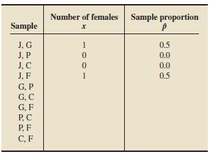
Repeat parts (b)–(e) of Exercise 11.9 for samples of size 4.(b)–(e) of Exercise 11.9b. The first column of the following table provides the possible samples of size 2, where each person is represented by the first letter of his or her first name; the second column gives the number of
Repeat parts (b)–(e) of Exercise 11.9 for samples of size 5.(b)–(e) of Exercise 11.9b. The first column of the following table provides the possible samples of size 2, where each person is represented by the first letter of his or her first name; the second column gives the number of
Hypothesis tests are proposed. For each hypothesis test,a. identify the variable.b. identify the two populations.c. determine the null and alternative hypotheses.d. classify the hypothesis test as two tailed, left tailed, or right tailed.Contingent faculty members in higher education are non-tenure
Multi-sensor data loggers were attached to free-ranging American alligators in a study conducted by Y. Watanabe for the article “Behavior of American Alligators Monitored by Multi-Sensor Data Loggers”. The mean duration for a sample of 68 dives was 338.0 seconds. Assume the population standard
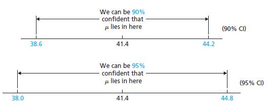
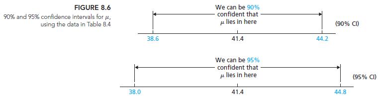
Refer to Exercise 8.77.a. Determine the margin of error for the 95% confidence interval.b. Determine the margin of error for the 90% confidence interval.c. Compare the margins of error found in parts (a) and (b).d. What principle is being illustrated?Exercise 8.77An issue with legalization of
American Alligators. Refer to Exercise 8.78.a. Determine the margin of error for the 95% confidence interval.b. Determine the margin of error for the 99% confidence interval.c. Compare the margins of error found in parts (a) and (b).d. What principle is being illustrated? Exercise
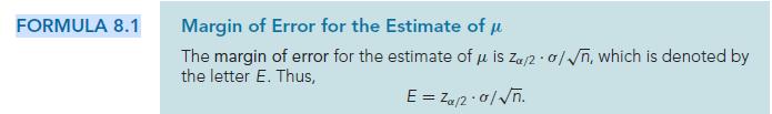
In Exercise 8.69, you found a 95% confidence interval for the mean amount of all venture-capital investments in the fiber optics business sector to be from $5.389 million to $7.274 million. Obtain the margin of error bya. Taking half the length of the confidence interval.b. Using Formula
You found a 95% confidence interval of 18.8 months to 48.0 months for the mean duration of imprisonment, μ, of all East German political prisoners withchronic PTSD.a. Determine the margin of error, E.b. Explain the meaning of E in this context in terms of the accuracy of the estimate.c. Find the
Another type of confidence interval is called a one-sided confidence interval. A one-sided confidence interval provides either a lower confidence bound or an upper confidence bound for the parameter in question. You are asked to examine one-sided confidence intervals.Presuming that the assumptions

Showing 600 - 700 of 1910

1
2
3
4
5
6
7
8
9
10
11
12
13
14
15
Last

Step by Step Answers

Services

Sitemap
Fun
Definitions
Become Tutor
Used Textbooks
Study Help Categories
Recent Questions
Expert Questions
Campus Wear
Sell Your Books

Company Info

Security
Copyrights
Privacy Policy
Terms & Conditions
SolutionInn Fee
Scholarship
Online Quiz
Give Feedback, Get Rewards

Get In Touch

About Us
Contact Us
Career
Jobs
FAQ
Student Discount
Campus Ambassador

Secure Payment

Download Our App

© 2026 SolutionInn. All Rights Reserved