New Semester Started Get 50% OFF Study Help! --h --m --s Claim Now

Question Answers

Textbooks

Find textbooks, questions and answers

Oops, something went wrong!

Change your search query and then try again

Result Not Found

Books FREE
Study Help
Tutors
AI Study Planner NEW
Sell Books

Search
Sign In
Register

study help
mathematics
advanced engineering mathematics

Advanced Engineering Mathematics 10th edition Erwin Kreyszig - Solutions

Let A = [αjk] be an n x n matrix with (not necessarily distinct) eigenvalues λ1, · · · , λn. Show.The sum of the main diagonal entries, called the trace of A, equals the sum of the eigenvalues of A.
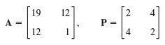
Verify that A and AÌ‚ = p-1AP have the same spectrum. 19 4 2 12 1 P.
This important concept denotes a matrix that commutes with its conjugate transpose AA̅T = A̅TA. Prove that Hermitian, skew-Hermitian, and unitary matrices are normal. Give corresponding examples of your own.
Do there exist non singular skew-symmetric n × n matrices with odd n?
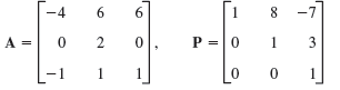
Verify that A and AÌ‚ = p-1AP have the same spectrum. -4 -7 P =|0 3 1 1
Let A = [αjk] be an n x n matrix with (not necessarily distinct) eigenvalues λ1, · · · , λn. Show.kA has the eigenvalues kλ1,· · ·, kλn. Am(m = 1, 2, · · ·) has the eigenvalues λ1m, · · ·,λnm. The eigenvectors are those of A.
Find an eigenbasis and diagonalize. 72 -56 - 56 513
Find the matrix A in the linear transformation y = Ax, where x = [x1 x2]T (x = [x1 x2 x3]T) are Cartesian coordinates. Find the eigenvalues and eigenvectors and explain their geometric meaning.Orthogonal projection of R3 onto the plane x2 = x1.
What kind of conic section (or pair of straight lines) is given by the quadratic form? Transform it to principal axes. Express xT = [x1 x2] in terms of the new coordinate vector yT = [y1 y2], as in Example 6.9x12 + 6x1x2 + x22 = 10
Do there exist nondiagonal symmetric 3 x 3 matrices that are orthogonal?
Find a simple matrix that is not normal. Find a normal matrix that is not Hermitian, skew-Hermitian, or unitary.
Transform to canonical form (to principal axes). Express [x1 x2]T in terms of the new variables [y1 y2]T..9x12 - 6x1x2 + 17x22 = 36
What kind of conic section (or pair of straight lines) is given by the quadratic form? Transform it to principal axes. Express xT = [x1 x2] in terms of the new coordinate vector yT = [y1 y2], as in Example 6.4x12 + 12x1x2 + 13x22 = 16
Transform to canonical form (to principal axes). Express [x1 x2]T in terms of the new variables [y1 y2]T.5x12 + 24x1x2 - 5x22 = 0
Show that A-1 exists if and only if the eigenvalues λ1, · · ·, λn are all nonzero, and then A-1 has the eigenvalues 1/λ1, · · ·,1/λn.
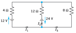
In Probs. 17€“19, using Kirchhoff€™s laws and showing the details, find the currents: 82 12 2 24 V 12 v
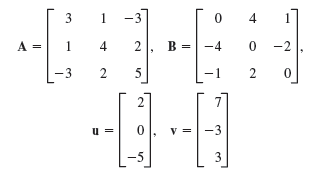
Showing the details, calculate the following expressions or give reason why they are not defined, when(A2)-1, (A-1)2 3 1 -3 4 1 2, B =-4 A = 4 -2 -3 2 V =-3
Showing all intermediate results, calculate the following expression or give reasons why they are undefined:ab, ba, aA, Bb Let 4 -2 3 -3 A =-2 1 B = -3 6. 1 2 2 -2 1. a = [1 -2 0], 0), b = 3 2 -2
By definition, forces are in equilibrium if their resultant is the zero vector. Find a force p such that the above u, v, w, and p are in equilibrium.
Same task as in Prob. 16 for the matrix in Prob. 7.Give an application of the matrix in Prob. 2 that makes the form of the inverse obvious.Data from Prob 2Find the inverse by Gauss€“Jordan (or by (4*) if n = 2). Check by using (1).Data from Prob 7Find the inverse by
Are the following sets of vectors linearly independent? Show the details of your work. 14
Find the Euclidean norm of the vectors:[-4 8 -1]T
Showing all intermediate results, calculate the following expression or give reasons why they are undefined:bTAb, aBaT, aCCT, CTba Let 4 -2 3 -3 A =-2 1 B = -3 6. 1 2 2 -2 1. a = [1 -2 0], 0), b = 3 2 -2
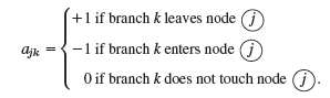
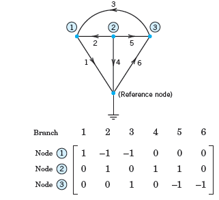
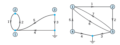
Matrices have various engineering applications, as we shall see. For instance, they can be used to characterize connections in electrical networks, in nets of roads, in production processes, etc., as follows.The network in Fig. 155 consists of six branches (connections) and four nodes (points where
Are the following sets of vectors linearly independent? Show the details of your work. [1 2 3 4], [2 3 4 5], [3 4 5 6]. 4 5 6 7]
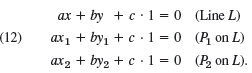
The idea is to get an equation from the vanishing of the determinant of a homogeneous linear system as the condition for a nontrivial solution in Cramer€™s theorem. We explain the trick for obtaining such a system for the case of a line L through two given points P1: (x1, y1) and P2: (x2,
Solve by Cramer’s rule. Check by Gauss elimination and back substitution. Show details.2x - 4y = -245x + 2y = 0
Determine the ranks of the coefficient matrix and the augmented matrix and state how many solutions the linear system will have.In Prob. 26Data from Prob. 26Showing the details, find all solutions or indicate that no solution exists. 2x + 3y - 7z = 3-4x - 6y + 14z = 7
Is the given set of vectors a vector space? Give reasons. If your answer is yes, determine the dimension and find a basis. (v1, v2, · · · denote components.)All vectors in R3 with 3v1 - 2v2 + v3 = 0, 4v1 + 5v2 = 0
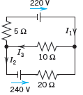
Find the currents. 220 V 10Ω (12 20 2 240 V
Are the given functions linearly independent or dependent on the half-axis x > 0? Give reason.cos2 x, sin2 x, 2π
Extend the method to Euler–Cauchy equations. Comment on the practical significance of such extensions.
Solve the following ODEs, showing the details of your work.y"' + 2y" - y' - 2y = 1 - 4x3
Solve the given ODE. Show the details of your work.yiv + 2y" + y = 0
Solve the following ODEs, showing the details of your work.(D3 + 3D2 - 5D – 39I)y = -300 cos x
Solve the given ODE. Show the details of your work.(D3 - D2 - D + l) y = 0
Solve the following ODEs, showing the details of your work.(D3 + 4D)y = sin x
Solve the given ODE. Show the details of your work.yiv - 3y" - 4y = 0
Solve the given ODE. Show the details of your work.(D5 + 8D3 + 16D)y = 0
Solve the given IVP, showing the details of your work.yiv - 5y" + 4y = l0e-3x, y(0) = 1, y' (0) = 0, y" (0) = 0, y"' (0) = 0
Are the given functions linearly independent or dependent on the half-axis x > 0? Give reason.x2, 1/x2, 0
Solve the given ODE. Show the details of your work.y"' - 4y" - y' + 4y = 30e2x
Solve the given IVP, showing the details of your work.x3y"' + xy' - y = x2, y(1) = 1, y' (1) = 3, y" (1) = 14
Are the given functions linearly independent or dependent on the half-axis x > 0? Give reason.e2x, xe2x, x2e2x
Solve the given ODE. Show the details of your work.x2y"' + 3xy" - 2y' = 0
Solve the given ODE. Show the details of your work.(D3 - D)y = sinh 0.8x
Are the given functions linearly independent or dependent on the half-axis x > 0? Give reason.sin2 x, cos2 x, cos 2x
Solve the given IVP, showing the details of your work.(D3 - 2D2 - 9D + 18I)y = e2x, y(0) = 4.5, y' (0) = 8.8, y" (0) = 17.2
Since variation of parameters is generally complicated, it seems worthwhile to try to extend the other method. Find out experimentally for what ODEs this is possible and for what not. Work backward, solving ODEs with a CAS and then looking whether the solution could be obtained by undetermined
Solve the given ODE. Show the details of your work.(D4 - 13D2 + 36I)y = 12ex
This is of practical interest since a single solution of an ODE can often be guessed.(a) How could you reduce the order of a linear constant-coefficient ODE if a solution is known?(b) Reduce x3y"' - 3x2y" + (6 - x2)xy' - (6 - x2)y = 0, using y1 = x (perhaps obtainable by inspection).
Solve the IVP. Show the details of your work.(D3 - D2 - D + I)y = 0, y(0) = 0, Dy(0) = 1, D2y(0) = 0
Solve the IVP. Show the details of your work.(D4 - 26D2 + 25I)y = 50(x + 1)2, y(0) = 12.16, Dy(0) = -6, D2y(0) = 34, D3y(0) = -130
Solve the IVP. Show the details of your work.(D3 + 3D2 + 3D + I)y = 8 sin x, y(0) = -1, y' (0) = -3, y" (0) = 5
Find a (real) general solution. State which rule you are using. Show each step of your work.(D2 + 2D + I)y = 2x sin x
Find an ODE y" + ay' + by = 0 for the given basis.cos 2πx, sin 2πx
If a body hangs on a spring s1 of modulus k1 = 8, which in turn hangs on a spring s2 of modulus k2 = 12, what is the modulus k of this combination of springs?
Find the Wronskian. Show linear independence by using quotients and confirm it by Theorem 2.e-x cos ωx, e-x sin ωx
Solve the given nonhomogeneous linear ODE by variation of parameters or undetermined coefficients. Show the details of your work.(D2 + 6D + 9I)y = 16e-3x/(x2 + 1)
Find a (real) general solution. State which rule you are using. Show each step of your work.y" + y' + (π2 + 1/4)y = e-x/2 sin πx
Find a real general solution. Show the details of your work.x2y" + 0.7xy' - 0.1y = 0
Could you make a harmonic oscillation move faster by giving the body a greater initial push?
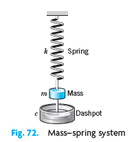
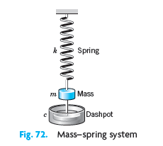
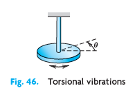
In Fig. 72, let m = 1 kg, c = 4 kg/sec, k = 24 kg/sec2, and r(t) = 10 cos ωt nt. Determine w such that you get the steady-state vibration of maximum possible amplitude. Determine this amplitude. Then find the general solution with this and check whether the results are in agreement. Spring m Mass
Find the motion of the mass??spring system in Fig. 72 with mass 0.125 kg, damping 0, spring constant 1.125 kg/sec2, and driving force cos t - 4 sin t nt, assuming zero initial displacement and velocity. For what frequency of the driving force would you get resonance? Spring | Mass m Dashpot Fig.
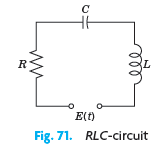
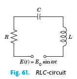
Find the current in the RLC-circuit in Fig. 71 when R = 40 Ω, L = 0.4 H, C = 10-4F, E = 220 sin 314t V (50 cycles/sec). R E(t) Fig. 71. RLC-circuit
Find a general solution of the homogeneous linear ODE corresponding to the ODE in Prob. 23. Data from Prob. 23 Find the steady-state current in the RLC-circuit in Fig. 71 when R = 2 kΩ (2000 Ω), L = 1 H, C = 4 ? 10-3 F, and E = 110 sin 415t V (66 cycles/sec). R E(t) Fig. 71. RLC-circuit
Solve the problem, showing the details of your work. Sketch or graph the solution.(x2D2 + 15xD + 49I)y = 0, y(1) = 2, y' (1) = -11
(a) Derive a second linearly independent solution of (1) by reduction of order; but instead of using (9), Sec. 2.1, perform all steps directly for the present ODE (1).(b) Obtain xm ln x by considering the solutions xm and xm+s of a suitable Euler–Cauchy equation and letting s → 0.(c) Verify by
Solve the problem, showing the details of your work. Sketch or graph the solution.y" - 3y' + 2y = 10 sin x, y(0) = 1, y' (0) = -6
Solve LI∼" + RI∼' + I∼/C = E0eiωt, i = √-1, by substituting lp = Keiωt (K unknown) and its derivatives and taking the real part lp of the solution l∼p. Show agreement with (2), (4). Use (11) eiωt = cos ωt + i sin ωt; cf. Sec. 2.2, and i2 = -1.
Solve the initial value problem. State which rule you are using. Show each step of your calculation in detail.(D2 + 2D + 10I)y = 17 sin x - 37 sin 3x, y(0) = 6.6, y' (0) = -2.2
Solve and graph the solution. Show the details of your work.(9x2D2 + 3xD + I)y = 0, y(1) = 1, y' (1) = 0
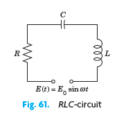
Solve the initial value problem for the RLC circuit in Fig. 61 with the given data, assuming zero initial current and charge. Graph or sketch the solution. Show the details of your work. R = 18 Ω, L = 1 H, C = 1.25 ? 10-3?F, E = 820 cos 10t V R L E(t) = E, sin ot Fig. 61. RLC-circuit
Find a general solution. Show the details of your calculation.yy" = 2y'2
Show that the maxima of an under damped motion occur at equidistant t-values and find the distance.
Find an ODE y" + ay' + by = 0 for the given basis.e2.6x, e-4.3x
Solve the initial value problem. State which rule you are using. Show each step of your calculation in detail.(D2 - 2D)y = 6e2x - 4e-2x, y(0) = -1, y' (0) = 6
Solve and graph the solution. Show the details of your work.(x2D2 - 3xD + 4I)y = 0, y(1) = -π, y' (1) = 2π
Solve the initial value problem for the RLC circuit in Fig. 61 with the given data, assuming zero initial current and charge. Graph or sketch the solution. Show the details of your work. R = 8 Ω, L = 0.2 H, C = 12.5 ? 10-3 F, E = 100 Sin 10t V R L E(t) = E, sin ot Fig. 61. RLC-circuit
Find a general solution. Show the details of your calculation.(D2 + 2D + 2I)y = 3e-x cos 2x
Find a general solution. Show the details of your calculation.(x2D2 + xD – 9I)y = 0
What is the smallest value of the damping constant of a shock absorber in the suspension of a wheel of a car (consisting of a spring and an absorber) that will provide (theoretically) an oscillationfree ride if the mass of the car is 2000 kg and the spring constant equals 4500 kg/sec2?
(a) Find a second-order homogeneous linear ODE for which the given functions are solutions. (b) Show linear independence by the Wronskian. (c) Solve the initial value problem.e-kx cos πx, e-kx sin πx, y(0) = 1 y' (0) = -k - π
The undetermined-coefficient method should be used whenever possible because it is simpler. Compare it with the present method as follows.(a) Solve y" + 4y' + 3y = 65 cos 2x by both methods, showing all details, and compare.(b) Solve y" - 2y' + y = r1 + r2, r1 = 35 x3/2 exr2 = x2 by applying each
Solve the initial value problem. State which rule you are using. Show each step of your calculation in detail.y" + 4y' + 4y = e-2x sin 2x, y(0) = 1, y' (0) = -1.5
Solve and graph the solution. Show the details of your work.x2y" + xy' + 9y = 0, y(1) = 0, y' (1) = 2.5
Find a general solution. Show the details of your calculation.(D2 + 4πD + 4π2I)y = 0
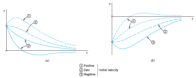
Show that in the overdamped case, the body can pass through y = 0 at most once (Fig. 37). (b) (a) (1) Positive (2) Zero Initial velocity Negative
(a) Find a second-order homogeneous linear ODE for which the given functions are solutions. (b) Show linear independence by the Wronskian. (c) Solve the initial value problem.x2, x2 lnx, y(1) = 4, y' (1) = 6
Solve the given nonhomogeneous linear ODE by variation of parameters or undetermined coefficients. Show the details of your work.(D2 - I)y = 1/cosh x
Solve the initial value problem. State which rule you are using. Show each step of your calculation in detail.y" + 4y = -12 sin 2x, y(0) = 1.8, y' (0) = 5.0
Solve and graph the solution. Show the details of your work.x2y " - 4xy' + 6y = 0, y(1) = 0.4, y' (1) = 0
Find the steady-state current in the RLC-circuit in Fig. 61 for the given data. Show the details of your work. R = 0.2 Ω, L = 0.1 H, C = 2 F, E = 220 sin 314t V L E(t) = E, sin ot Fig. 61. RLC-circuit
Find a general solution. Show the details of your calculation.y" + 0.20y' + 0.17y = 0
The unifying power of mathematical methods results to a large extent from the fact that different physical (or other) systems may have the same or very similar models. Illustrate this for the following three systems (a) Pendulum clock. A clock has a 1-meter pendulum. The clock ticks once for each
(a) Find a second-order homogeneous linear ODE for which the given functions are solutions. (b) Show linear independence by the Wronskian. (c) Solve the initial value problem.xm1, xm2, y(1) = -2, y' (1) = 2m1 - 4m2
Solve the given nonhomogeneous linear ODE by variation of parameters or undetermined coefficients. Show the details of your work.(D2 + 2D + 2I)y = 4e-x sec3x
Find a real general solution. Show the details of your work.(x2D2 - xD + 5I)y = 0
Find a general solution. Show the details of your calculation.y" + y' - 12y = 0
Find the Wronskian. Show linear independence by using quotients and confirm it by Theorem 2.xk cos (In x), xk sin (In x)

Showing 3700 - 3800 of 3937

First
26
27
28
29
30
31
32
33
34
35
36
37
38
39
40

Step by Step Answers

Services

Sitemap
Fun
Definitions
Become Tutor
Used Textbooks
Study Help Categories
Recent Questions
Expert Questions
Campus Wear
Sell Your Books

Company Info

Security
Copyrights
Privacy Policy
Terms & Conditions
SolutionInn Fee
Scholarship
Online Quiz
Give Feedback, Get Rewards

Get In Touch

About Us
Contact Us
Career
Jobs
FAQ
Student Discount
Campus Ambassador

Secure Payment

Download Our App

© 2026 SolutionInn. All Rights Reserved