New Semester
Started
Get
50% OFF
Study Help!
--h --m --s
Claim Now
Question Answers
Textbooks
Find textbooks, questions and answers
Oops, something went wrong!
Change your search query and then try again
S
Books
FREE
Study Help
Expert Questions
Accounting
General Management
Mathematics
Finance
Organizational Behaviour
Law
Physics
Operating System
Management Leadership
Sociology
Programming
Marketing
Database
Computer Network
Economics
Textbooks Solutions
Accounting
Managerial Accounting
Management Leadership
Cost Accounting
Statistics
Business Law
Corporate Finance
Finance
Economics
Auditing
Tutors
Online Tutors
Find a Tutor
Hire a Tutor
Become a Tutor
AI Tutor
AI Study Planner
NEW
Sell Books
Search
Search
Sign In
Register
study help
statistics
elementary statistics in social research
Elementary Statistics In Social Research 12th Edition Jack A. Levin, James Alan Fox, David R. Forde - Solutions
For the exponential family of distributions defined in (4.41), show(a) \(E(y)=\frac{d}{d \theta} b(\theta)\).(b) \(\operatorname{Var}(y)=a(\phi) \frac{d^{2}}{d \theta^{2}} b(\theta)\).(c) Assume that \(y \sim N\left(\mu, \sigma^{2}\right)\) and \(\sigma^{2}\) is known. Show that the canonical link
Prove that a sufficient statistic for the parameter \(\beta_{j}\) in the model (4.25) is given by \(T_{j}(x)=\sum_{i=1}^{n} y_{i} x_{i j}(1 \leq j \leq p)\). logit (T) = log = Box10 + + BpTip = Tx. (4.25) i
This problem illustrates why exact inference may not behave well when conditional on continuous covariates.(a) Consider the following equation where \(a_{1}, a_{2}, \ldots, a_{n}\) are some known numbers and \(y_{i}\) are binary variables,\[\begin{equation*}\sum_{i=1}^{n} y_{i} a_{i}=0, \quad y_{i}
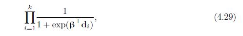
Verify the conditional likelihood (4.29). k II i=1 1 1+ exp( d;)' (4.29)
Suppose \(y_{i}=\sum_{j=1}^{n_{i}} y_{i j}\), where \(y_{i j} \sim \operatorname{Bernoulli}\left(p_{i}\right)\) and are positively correlated with \(\operatorname{cor}\left(y_{i j}, y_{i k}\right)=\alpha>0\) for \(k eq j\). Prove \(\operatorname{Var}\left(y_{i}\right)>n_{i}
Prove that the deviance and Pearson chi-square test statistics are asymptotically equivalent.
Plot and compare the CDFs of logistic, probit, and complementary log-log variables after they are centered at their medians and scaled to unit variances.
Let \(y_{i}^{*}=\beta_{0}+\boldsymbol{\beta}^{\top} \mathbf{x}_{i}+\varepsilon_{i}\), where \(\varepsilon_{i} \sim N(0,1)\) (a standard normal with mean 0 and variance 1 ) and \(y_{i}\) is determined by \(y_{i}^{*}\) as an indicator for whether this latent variable is positive, i.e.,\[y_{i}=
Prove that if\[\operatorname{Pr}\left(y_{i}=1 \mid \mathbf{x}_{i}\right)=\Phi\left(\beta_{0}+\mathbf{x}^{\top} \boldsymbol{\beta}\right), \quad \operatorname{Pr}\left(y_{i}=0 \mid \mathbf{x}_{i}\right)=\Phi\left(\alpha_{0}+\mathbf{x}^{\top} \boldsymbol{\alpha}\right)\]where \(\Phi\) is the CDF of
Fit complementary log-log models to DOS data, using dichotomized depression as response and gender as the predictor. Comparing the results between modeling the probability of No depression and modeling the probability of Depression. This confirms that the complementary log-log link function is not
Use the baseline information from the Catheter Study. We model the binary catheter blockage outcome with age, gender, and education as predictors. Assuming additive effect for all these covariates, we may have five models using the four link functions: logit, probit, c-log-log, and identity. Note
Show that the discrimination slope equals to the differences of the mean fitted probabilities between \(y=1\) and \(y=0\).
For the Catheter Study, apply the binomial regression model (4.49) with the UTI response replaced by the catheter blockage.(a) What conclusions you may have based on the model? Is there overdispersion?(b) Apply the scaling approach to deal with the overdispersion issue. Are there any changes in
In this problem, we perform a simulation study about clustered binary outcomes with sample size 1000 .(a) Generate random variable \(X\) from \(\mathrm{N}(0,1)\).(b) For each \(X\), generate five binary responses with response probability \(\frac{\exp (x)}{1+\exp (x)}\) in two scenarios and sum up
Show that for a generalized logit model, \(T_{j k}(x)=\sum_{i=1}^{n} y_{i j} x_{i k}\) is a sufficient statistic for parameter \(\beta_{j k}(1 \leq j \leq J\) and \(1 \leq k \leq p)\).
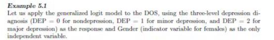
Compute the fitted probabilities for females based on the generalized logistic model in Example 5.1. Example 5.1 Let us apply the generalized logit model to the DOS, using the three-level depression di- agnosis (DEP 0 for nondepression, DEP 1 for minor depression, and DEP 2 for major depression) as
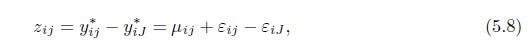
Prove that the multinomial probit model defined in (5.8) does not depend on the selection of the reference level. = zij ij Yi = Hij + Eij EiJ, (5.8)
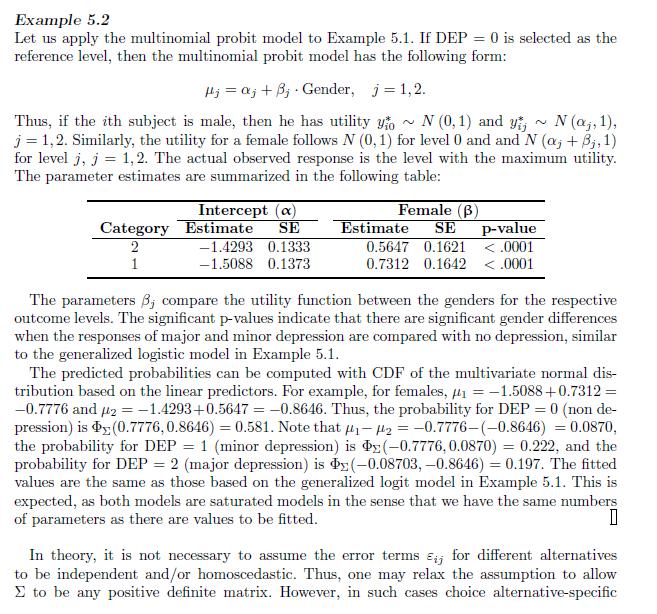
Compute the fitted probabilities for females based on the multinomial probit model in Example5.2 Example 5.2 Let us apply the multinomial probit model to Example 5.1. If DEP = 0 is selected as the reference level, then the multinomial probit model has the following form: Hja; ; Gender, j = 1,2. ~ N
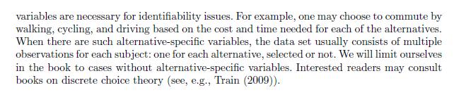
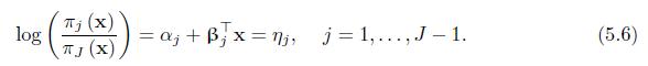
Prove that the generalized logit model (5.6) can be defined with utility functions \(y_{i j}^{*}=\alpha_{j}+\boldsymbol{\beta}_{j}^{\top} \mathbf{x}+\varepsilon_{i j}\), where \(\varepsilon_{i j}\) follows the standard Gumbel distribution for each level \(j=1, \ldots, J\) and for subjects \(i=1,
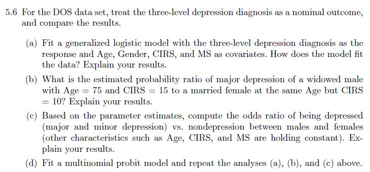
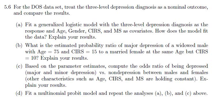
For the DOS data set, treat the three-level depression diagnosis as a nominal outcome, and compare the results.(a) Fit a generalized logistic model with the three-level depression diagnosis as the response and Age, Gender, CIRS, and MS as covariates. How does the model fit the data? Explain your
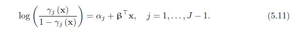
Verify (5.13) for the proportional odds model defined in (5.11). Yi (x1) / (1 Yi (x1)) Yi (x2)/(1-j (x2)) P (BT = exp (B (x1 -x2)), j=1,...,J 1. (5.13)
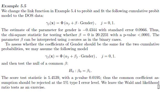
Find the Wald and LR test statistics for testing equality of slopes in Example5.5 Example 5.5 We change the link function in Example 5.4 to probit and fit the following cumulative probit model to the DOS data: (x)=(a+3 Gender), j=0,1. The estimate of the parameter for gender is -0.4344 with
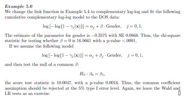
Find the Wald and LR test statistics for testing equality of slopes in Example5.6 Example 5.6 We change the link function in Example 5.4 to complementary log-log and fit the following cumulative complementary log-log model to the DOS data: log log{1-(x)}]=a, +3. Gender, j = 0,1. The estimate of the
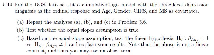
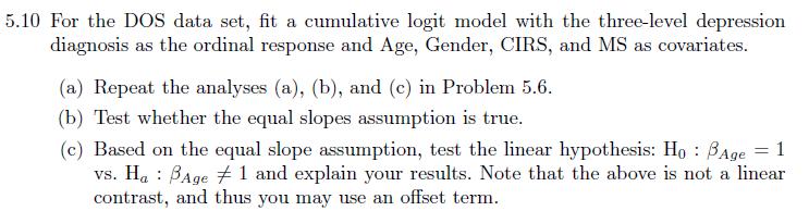
For the DOS data set, fit a cumulative logit model with the three-level depression diagnosis as the ordinal response and Age, Gender, CIRS, and MS as covariates.(a) Repeat the analyses (a), (b), and (c) in Problem5.6(b) Test whether the equal slopes assumption is true.(c) Based on the equal slope
Repeat the analyses in Problem5.10 with continuation ratio models with logit, probit, and complementary log-log link functions. Problem5.10 5.10 For the DOS data set, fit a cumulative logit model with the three-level depression diagnosis as the ordinal response and Age, Gender, CIRS, and MS as
Compute the correlation matrix of the fitted probabilities for having major depression based on the models in Problems 5.6, 5.10, 5.11, 5.12, and 5.13.Problems 5.6:Problems 5.10:Problems 5.11:Problems 5.12:Problems 5.13: 5.6 For the DOS data set, treat the three-level depression diagnosis as a
For an \(I \times J\) contingency table with ordinal column variable \(y(=1, \ldots, J)\) and ordinal row variable \(x(=1, \ldots, I)\), consider the model\[\operatorname{logit}[\operatorname{Pr}(y \leq j \mid x)]=\alpha_{j}+\beta x, j=1, \ldots, J-1\](a) Show that logit \([\operatorname{Pr}(y \leq
For an \(I \times J\) contingency table with ordinal column variable \(y(=1, \ldots, J)\) and ordinal row variable \(x(=1, \ldots, I)\), consider the adjacent category model\[\log \left[\frac{\operatorname{Pr}(y=j+1 \mid x)}{\operatorname{Pr}(y=j \mid x)}\right]=\alpha_{j}+\beta x, j=1, \ldots,
Show that the log function in (6.2) is the canonical link for the Poisson model in (6.1). Yi Xi ~ Poisson (#), 1 in. (6.1)
Consider a Poisson regression model for a count response \(y\) with a single continuous covariate \(x, E(y \mid x)=\exp \left(\alpha_{0}+\alpha_{1} x\right)\). If \(x\) is measured on another scale \(x^{\prime}\) such that \(x^{\prime}=k x\), and the model expressed in terms of \(x^{\prime}\) is
Show that for the Poisson regression model in (6.2), \(\sum_{i=1}^{n} y_{i} x_{i j}\) is a sufficient statistic for \(\beta_{j}(1 \leq j \leq p)\). log()=xB=Bxi1+...+pip (6.2)
Similar to logistic regression, give a definition of median unbiased estimate (MUE) of a parameter based on the exact conditional distribution.
Let \(y \sim \operatorname{Poisson}(\mu)\).(a) If \(\mu=n\) is an integer, show that the normalized variable \(\frac{y-\mu}{\sqrt{\mu}}\) has an asymptotic normal distribution \(N(0,1)\), i.e., \(\frac{y-\mu}{\sqrt{\mu}} \sim_{a} N(0,1)\) as \(\mu\rightarrow \infty\).(b) Generalize the conclusion
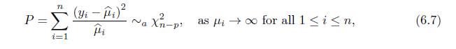
Show that the asymptotic result in (6.7) still holds if \(\beta\) is replaced by the MLE \(\widehat{\beta}\). n P = i=1 (Yi - ) D~ Xn-p as for all 1
For the Sexual Health pilot study, consider modeling the number of unprotected vaginal sex behaviors during the three month period of the study as a function of three predictors, HIV knowledge, depression, and baseline number of unprotected vaginal sex (VAGWOCT1).(a) Fit the Poisson log-linear
Use the intake data for the Catheter Study to study the association between urinary tract infection (UTI) and demographic characteristics including age, gender, and marital status (ms). There are seven levels for the \(\mathrm{ms}\) in the original data, and we combine levels 2 to 6 to make it a
Prove that the CMP distribution \(\operatorname{CMP}(\lambda, v)\) converges to(a) a Bernoulli distribution as \(v\) goes to infinite. Find the parameter for the limiting Bernoulli distribution;(b) a geometric distribution as \(v \rightarrow 0\). Find the parameter for the limiting geometric
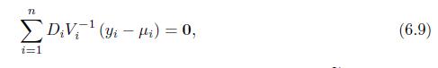
Consider the Poisson log-linear model\[y_{i} \mid \mathbf{x}_{i} \sim \text { Poisson }\left(\mu_{i}\right), \quad \log \left(\mu_{i}\right)=\mathbf{x}_{i}^{\top} \boldsymbol{\beta}, \quad 1 \leq i \leq n\]Show that the score equations have the form (6.9), with \(D_{i}=\frac{\partial
Show that inference about \(\beta\) based on \(\mathrm{EE}\) is valid even when the NB model does not describe the distribution of the count variable \(y_{i}\), provided that the systematic component \(\log \left(\mu_{i}\right)=\mathbf{x}_{i}^{\top} \boldsymbol{\beta}\) specified in (6.22) is
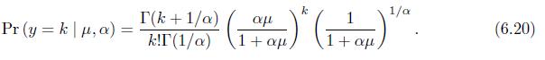
Let \(y\) follow the negative binomial distribution (6.20). Show that \(E(y)=\mu\) and \(\operatorname{Var}(y)=\mu(1+\alpha \mu)\), where \(\alpha\) is the dispersion parameter for the negative binomial distribution. 1/a T(k+1/a) == Pr(y kp, a) = k!I (1/a) (1 (6.20) 1 + 1 +
Let \(y\) follow a mixture of structural zeros of probability \(p\) and a Poisson distribution with mean \(\mu\) of probability \(q=1-p\). Show that \(E(y)=q \mu\), and \(\operatorname{Var}(y)=q \mu+p q \mu^{2}\). Thus, the variance of a ZIP outcome variable is always larger than its mean, and the
Have you experienced Simpson's paradox in your professional and/or personal life? If so, please describe the context in which it occurred.
Suppose you test ten hypotheses and under the null hypothesis each hypothesis is to be rejected with type I error rate 0.05. Assume that the hypotheses (test statistics) are independent. Compute the probability that at least one hypothesis will be rejected under the null hypothesis.
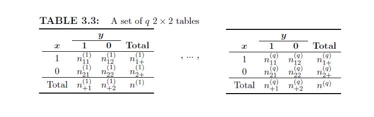
Show that the asymptotic distribution for the CMH test for a set of \(q 2 \times 2\) tables is valid as long as the total size is large. More precisely, (Q_{CMH}\rightarrow_{d}N(0,1)\)if(\Sigma_{i=1}^{q} n^{(h)}\rightarrow\) \(\infty\). TABLE 3.3: A set of q 2 x 2 tables y 1 0 Total (1) (1) (1) 1
Let \(\mathbf{x}\) be a random vector and \(\boldsymbol{V}\) its variance matrix. Show that \(\mathbf{x}^{\top} \boldsymbol{V}^{-1} \mathbf{x}\) is invariant under linear transformation. More precisely, let \(\boldsymbol{A}\) be some nonsingular square matrix, \(\mathbf{x}^{\prime}=\boldsymbol{A}
Use the DOS data to test whether there is gender and depression (dichotomized according to no and minor/major depression) association by stratifying medical burden and education levels, where medical burden has two levels (CIRS \(\leq 6\) and \(\operatorname{CIRS}>6\) ) and education has two levels
Show that the odds ratio is a monotone function of \(p_{11}\) if marginal distributions are fixed.
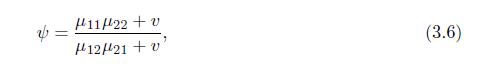
Verify (3.6) . H1122+v #1221 +v (3.6)
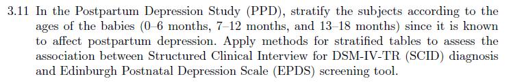
In the Postpartum Depression Study (PPD), stratify the subjects according to the ages of the babies (0-6 months, 7-12 months, and 13-18 months) since it is known to affect postpartum depression. Apply methods for stratified tables to assess the association between Structured Clinical Interview for
Redo Problem 2.16 by stratifying the subjects according to baby ages as in Problem 3.11Problem 2.16Problem 3.11 2.16 In the PPD, each subject was diagnosed for depression using SCID along with several screening tests including EPDS. By repeatedly dichotomizing the EPDS outcome, answer the following
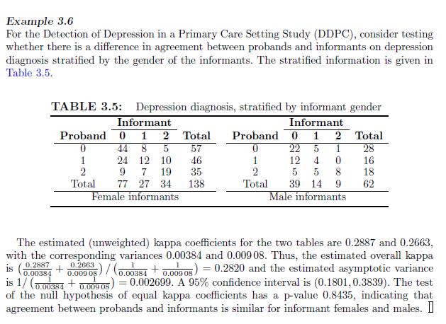
Use statistic software to verify the given estimates of (unweighted) kappa coefficients and their variances in Example3.6 for the two individual tables in Table3.5 Example 3.6 For the Detection of Depression in a Primary Care Setting Study (DDPC), consider testing whether there is a difference in
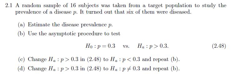
A random sample of 16 subjects was taken from a target population to study the prevalence of a disease \(p\). It turned out that six of them were diseased.(a) Estimate the disease prevalence \(p\).(b) Use the asymptotic procedure to test\[\begin{equation*}H_{0}: p=0.3 \quad \text { vs. } \quad
Since the sample size in Problem 2.1 is not very large, it is better to use exact tests.(a) Apply exact tests to test the hypothesis in (2.48) for the data in Problem 2.1 and compare your results with those derived from asymptotic tests.(b) Change \(H_{a}: p>0.3\) in (2.48) to \(H_{a}: p(c)
Check that in the binary case \((k=2)\), the statistic in (2.7) is equivalent to the one in (2.1).
In the DOS, we are interested in testing the following hypothesis concerning the distribution of depression diagnosis for the entire sample:\[\begin{aligned}\operatorname{Pr}(\text { No depression }) & =0.5 \\\operatorname{Pr}(\text { Minor depression }) & =0.3 \\\operatorname{Pr}(\text { Major
Suppose \(x \sim B I(n, p)\) follows a binomial distribution of size \(n\) and probability \(p\). Let \(k\) be an integer between 0 and \(n\). Show that \(\operatorname{Pr}(x \geq k)\), looking as a function of \(p\) with \(n\) and \(k\) fixed, is an increasing function of \(p\).
Prove that(a) If \(y \sim \operatorname{Poisson}(\lambda)\), then both the mean and variance of \(y\) are \(\lambda\).(b) If \(y_{1}\) and \(y_{2}\) are independent and \(y_{j} \sim \operatorname{Poisson}\left(\lambda_{j}\right)(j=1,2)\), then the sum \(y_{1}+y_{2}
Following the MLE method, the information matrix is closely related with the asymptotic variance of MLE. For the MLE of Poisson distribution,(a) First compute the Fisher information matrix then plug in the MLE \(\hat{\lambda}\) to estimate the variance of \(\widehat{\lambda}\).(b) Plug in
Derive the negative binomial (NB) distribution.(a) Suppose \(y\) follows a Poisson \((\lambda)\), where the parameter \(\lambda\) itself is a random variable following a gamma distribution \(\operatorname{Gamma}(p, r)\). Derive the distribution of \(y\). (Note that the density function of a
Prove the equation below (2.11). - P11 P1+P+1 ~a N (P11 P1+P+1, [P+P+1 (1 P1+) (1 P+1)]). (2.11) n
Consider the statistic in (2.14).(a) Show that this statistic is asymptotically normal with the asymptotic variance given by\[\operatorname{Var}_{a}\left(\sqrt{n}\left(\widehat{p}_{1}-\widehat{p}_{2}\right)\right)=\frac{n}{n_{1+}} p_{1}\left(1-p_{1}\right)+\frac{n}{n_{2+}} p_{2}\left(1-p_{2}\right)
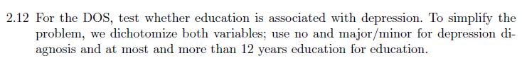
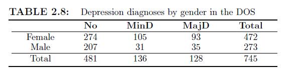
For the DOS, test whether education is associated with depression. To simplify the problem, we dichotomize both variables; use no and major/minor for depression diagnosis and at most and more than 12 years education for education.
Derive the relationships among the eight versions of odds ratios of Section 2.2.2.When twovariables(orrowandcolumn)areactuallyassociated,wemaywanttoknowthenature oftheassociation.Therearemanyindicesthathavebeendevelopedtocharacterizethe
Let \(p_{1}=\operatorname{Pr}(y=1 \mid x=1)=0.8\) and \(p_{2}=\operatorname{Pr}(y=1 \mid x=0)=0.4\).(a) Compute the relative risk of response \(y=1\) of population \(x=1\) to population \(x=0\), and the relative risk of response \(y=0\) of population \(x=1\) to population \(x=0\).(b) Change the
Show that the hypergeometric distribution \(H G\left(k ; n, n_{1+}, n_{+1}\right)\) has mean \(\frac{n_{1+} n_{+1}}{n}\) and variance \(\frac{n_{1+} n_{+1} n_{+2} n_{2+}}{n^{2}(n-1)}\).
In the PPD, each subject was diagnosed for depression using SCID along with several screening tests including EPDS. By repeatedly dichotomizing the EPDS outcome, answer the following questions:(a) For all possible EPDS cut-points observed in the data, compute the kappa coefficients between SCID and
The data set "intake" contains baseline information of the Catheter Study. Use the two binary outcomes on whether urinary tract infections (UTIs) and catheter blockages occurred during the last two months to assess(a) whether catheter blockage is associated with UTI;(b) the relative risk and odds
Group the count responses on UTIs and catheter blockages in the data set "intake" into three levels: no occurrence, only once, and more than once. Use these three-level outcomes to assess(a) whether catheter blockage is associated with UTI;(b) whether catheter blockage and UTI have the same
For the DOS, use the three-level depression diagnosis and dichotomized education (more than 12 years education or not) to check the association between education and depression.(a) Test whether education and depression are associated;(b) Compare the results of part(a) with that from Problem 2.12.
The data set "DosPrepost" contains depression diagnosis of patients at baseline (pretreatment) and one year after treatment (posttreatment) in the DOS. We are interested in whether there is any change in depression rates between pre- and post treatment.(a) Carry out the two-sided asymptotic and
Let \(p\) denote the prevalence of a disease of interest. Express \(P P V\) and \(N P V\) as a function of \(p, S e\), and \(S p\).
Prove that the weighted kappa for \(2 \times 2\) tables will reduce to the simple kappa, no matter which weights are assigned to the two levels.
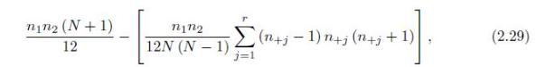
Verify the variance formula for the MWW statistics (2.29). nin2 (N+1) 12 r 12N (N-1) (n+j - 1) n+j (n+j+1) (2.29) j=1
Use the three-level depression diagnosis and dichotomized education (more than 12 years education or not) in the DOS data to test the association between education and depression.(a) Use the Pearson chi-square statistic for the test;(b) Use the row mean score test;(c) Use the Pearson correlation
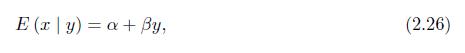
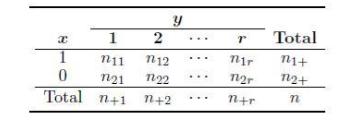
For the \(2 \times r\) table with scores as in Section 2.3.1,(a) verify that the MLE of \(\beta\) in the linear regression model in (2.26) is \(\widehat{\beta}=\frac{\overline{x y}-\bar{x} \bar{y}}{\bar{y}^{2}-\bar{y}^{2}}\);(b) prove \(E(x y)-E(x) E(y)=\sum_{j=1}^{r} p_{1
For the DOS, compute the indices, Pearson correlation, Spearman correlation, Goodman-Kruskal \(\gamma\), Kendall's \(\tau_{b}\), Stuart's \(\tau_{c}\), Somers' D, lambda coefficients, and uncertainty coefficients, for assessing association between education (dichotomized with cut-point 12) and
Many measures of association for two-way frequency tables consisting of two ordinal variables are based on the numbers of concordant and discordant pairs. To compute such indices, it is important to count each concordant (discordant) pair exactly once with no misses and repetitions. In Section
Suppose \(x\) is a random variable with \(m\) levels such that \(\operatorname{Pr}(x=i)=p_{i}\) for \(i=\) \(1,2, \ldots, m\) with \(\sum_{i=1}^{m} p_{i}=1\). In other words, \(x \sim \mathrm{MN}(1, \mathbf{p})\). Let \(x_{1}\) and \(x_{2}\) be two independent random variables following the
Let \(x\) be a binary variable with outcomes 0 and 1 . Let \(p=\operatorname{Pr}(x=1)\). Show that entropy has the maximum at \(p=0.5\).
For an \(r \times s\) table, the probability of concordant (discordant) pair \(p_{s}\left(p_{d}\right) \leq \frac{m-1}{m}\), where \(m=\min (r, s)\).
EPDS is an instrument (questionnaire) for depression in postpartum women. This instrument is designed so that a person with a higher EPDS score has a higher chance to be depressed. Use the PPD data to confirm this defining property of the instrument. More specifically,(a) Use the Cochran-Armitage
Suppose \(x\) is a random variable with at least two levels, with \(\operatorname{Pr}\left(x=x_{i}\right)=p_{i}\), for \(i=1,2\). Let \(x^{\prime}\) be the new random variable based on \(x\) with the two levels \(x_{1}\) and \(x_{2}\) combined, i.e.,\[x^{\prime}=\left\{\begin{array}{l}x_{1} \text {
If a fair die is thrown, then each number from 1 to 6 has the same chance of being the outcome. Let \(X\) be the random variable to indicate whether the outcome is 5, i.e.,\[X=\left\{\begin{array}{l}1 \text { if the outcome is } 5, \\0 \text { if the outcome is not } 5 .\end{array}\right.\](a)
For random variables \(X\) and \(Y\), show that \(E[E(X \mid Y)]=E(X)\) and \(\operatorname{Var}(X)=\operatorname{Var}(E(X \mid Y))+E(\operatorname{Var}(X \mid Y))\).
The sequence \(\left\{\frac{1}{n}\right\}_{n=1}^{\infty}\) converges to 0 . If we treat each constant, \(\frac{1}{n}\), as a constant random variable, then the corresponding \(\mathrm{CDF}\) is\[F_{n}(x)=\left\{\begin{array}{l}0 \text { if } x
Suppose \(X_{n} \sim \chi_{n}^{2}\), the chi-square with \(n\) degrees of freedom. Show that\[\frac{1}{\sqrt{2 n}}\left(X_{n}-n\right) \rightarrow_{d} N(0,1)\]
Let \(X_{1}, \ldots, X_{n}\), be a sequence of i.i.d. random variables that follow the Poisson distribution with mean \(\mu\). Then the sample average \(\bar{X}_{n}=\frac{X_{1}+\cdots+X_{n}}{n}\) is a consistent estimate of \(\mu\) and \(\bar{X}_{n}^{2}\) is a consistent estimate of \(\mu^{2}\).(a)
Prove Slutsky's theorem.
Prove that under some regularity conditions such as the exchangeability of the integral and differentiation, we have(a) \(E\left[\frac{1}{f\left(X_{i}, \boldsymbol{\theta}\right)} \frac{\partial}{\partial \boldsymbol{\theta}} f\left(X_{i}, \boldsymbol{\theta}\right)\right]=\mathbf{0}\). This shows
A random variable \(X\) follows an exponential distribution with parameter \(\lambda\) that takes positive values and \(\operatorname{Pr}(X
For an independent sample of \(Y_{i}\) and \(X_{i}(1 \leq i \leq n)\), suppose that\[\begin{equation*}Y_{i}=\mathbf{X}_{i}^{\top} \beta+\epsilon_{i}, \quad \epsilon_{i} \sim\left(0, \sigma_{i}^{2}\right), \quad 1 \leq i \leq n \tag{1.28}\end{equation*}\]where
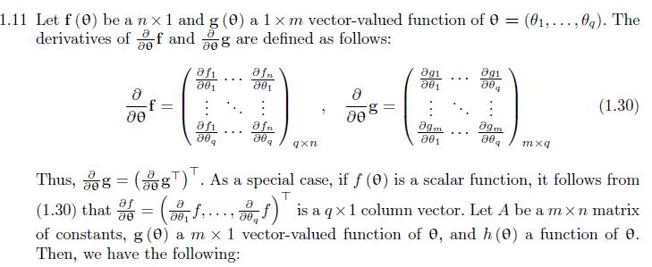
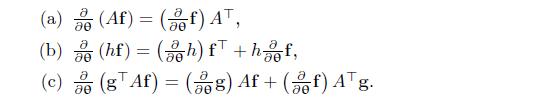
Let \(\mathbf{f}(\boldsymbol{\theta})\) be a \(n \times 1\) and \(\mathbf{g}(\boldsymbol{\theta})\) a \(1 \times m\) vector-valued function of \(\boldsymbol{\theta}=\left(\theta_{1}, \ldots, \theta_{q}\right)\). The derivatives of \(\frac{\partial}{\partial \boldsymbol{\theta}} \mathbf{f}\) and
Use the properties of differentiation in Problem1.11 to prove (1.13) and (1.14).Problem1.11 To prove (1.13) and (1.14). 1.11 Let f (0) be an x1 and g (0) a 1 xm vector-valued function of 0 = (01,..., 0q). The derivatives off and g are defined as follows: afi afn 01 801 f= 80 afi afn 80 qxn 1
Prove (1.21). ZEEE = E- (XX) E [X; (Y; X] B) X] E (X;X). - (1.21) n
Let \(\mathbf{X}_{i}(1 \leq i \leq n)\) be an i.i.d. sample of random vectors and let \(\mathbf{h}\) be a vector-valued symmetric function \(m\) arguments. Then,\[\widehat{\boldsymbol{\theta}}=\left(\begin{array}{c}n \\m\end{array}\right)^{-1} \sum_{\left(i_{1}, \ldots, i_{m}\right) \in C_{m}^{n}}
Show that the U-statistic \(\widehat{\sigma}^{2}\) in (1.24) is the sample variance of \(\sigma^{2}\), i.e., \(\widehat{\sigma}^{2}\) can be expressed as \(\widehat{\sigma}^{2}=\frac{1}{n-1} \sum_{i=1}^{n}\left(X_{i}-\bar{X}_{n}\right)^{2}\).
Consider the function \(\mathbf{h}\left(\mathbf{Z}_{1}, \mathbf{Z}_{2}\right)\) for the U-statistic in (1.22).(a) Show\[\operatorname{Var}\left[\widetilde{\mathbf{h}}_{1}\left(\mathbf{Z}_{1}\right)\right]=E\left(\mathbf{h}_{1}\left(\mathbf{Z}_{1}\right)
Let \(\mathbf{X}_{i}(1 \leq i \leq n)\) and \(\mathbf{Y}_{i}(1 \leq i \leq n)\) be two independent i.i.d. samples of random vectors from two different population. Let \(\mathbf{h}\) be a vector-valued symmetric function with \(s+t\) arguments. Show
Install the statistical software packages that you will use for the book in your computer. Read the DOS data set using your statistical software and find out the number of observations and the number of variables in the data sets.
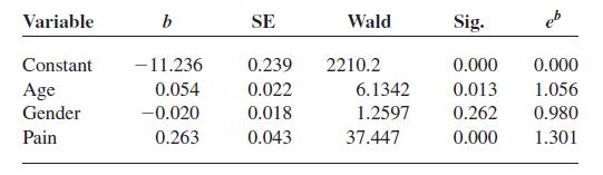
Referring back to Problem 19, the same doctor then used the three variables—pain level (pain), age, and gender—to predict whether or not patients were admitted to the hospital 1admit = 12 by the ER or sent home 1admit = 02. She performs a logistic regression which produces the following
Showing 1600 - 1700
of 1977
First
6
7
8
9
10
11
12
13
14
15
16
17
18
19
20
Step by Step Answers