New Semester Started Get 50% OFF Study Help! --h --m --s Claim Now

Question Answers

Textbooks

Find textbooks, questions and answers

Oops, something went wrong!

Change your search query and then try again

Result Not Found

Books FREE
Study Help
Tutors
AI Study Planner NEW
Sell Books

Search
Sign In
Register

study help
statistics
elementary statistics in social research

Applied Categorical And Count Data Analysis 2nd Edition Wan Tang, Hua He, Xin M. Tu - Solutions

Suppose \(x \sim N\left(0, u^{2}\right), y \sim N\left(0, \sigma^{2}\right)\), and \(x\) is independent of \(y\). Given \(x+y=1\), find the MLE for \(x\).
In this question we develop a regression model to assess the treatment effect for stigma in the DTS study, controlling for demographics and baseline measurements. We will use the cumulative logit link functions for the four-level stigma outcome and apply some model selection criteria to trim the
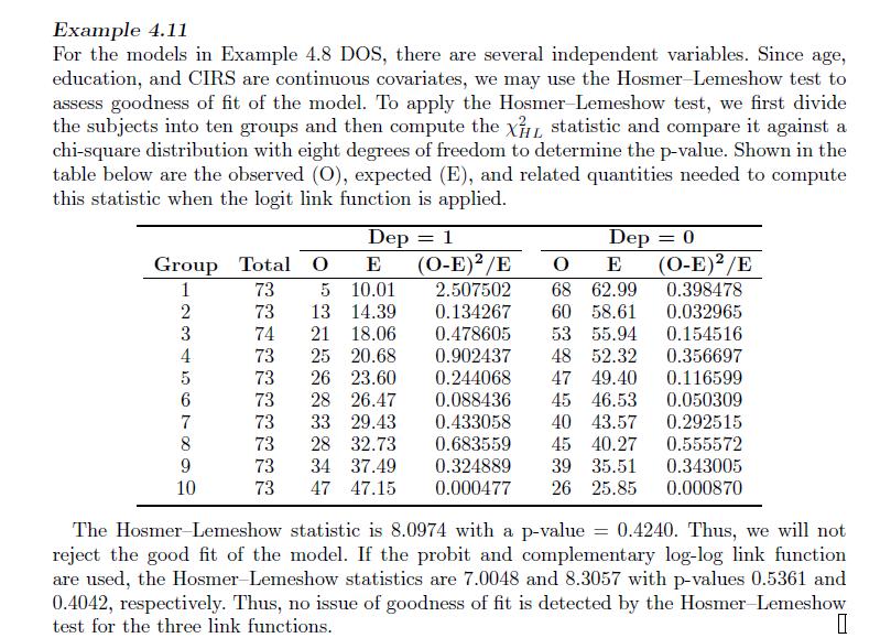
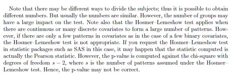
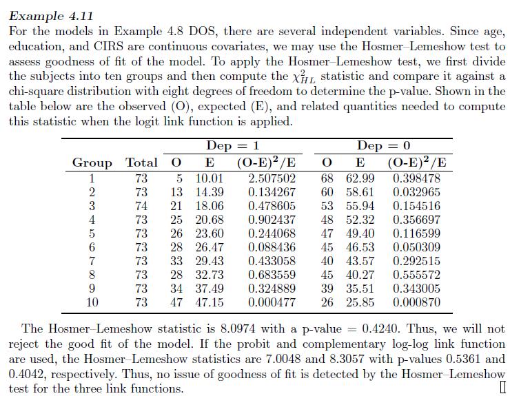
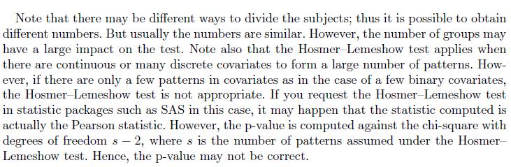
Generalize the model considered in Example 4.11 to a marginal model for the longitudinal DOS data and compare the findings with that in Example4.11 Example 4.11 For the models in Example 4.8 DOS, there are several independent variables. Since age, education, and CIRS are continuous covariates, we
Prove (9.31) . = BE (GS;S; G) BT, B = (B), B-T (9.31)
Show that \(\mathbf{x}_{i} \perp y_{i t} \mid \mathbf{x}_{i t}\) and \(E\left(y_{i t} \mid \mathbf{x}_{i t}\right)=\mu_{i t}\) imply the FCCM.
Consider the GLMM in (9.11) with a logit link. Show that(a) \(E\left(y_{i t} \mid \mathbf{x}_{i t}, \mathbf{z}_{i t}\right) \approx \Phi\left(\frac{\mathbf{x}_{i t}^{\top} \beta}{\sqrt{c^{2}+\mathbf{z}_{i t}^{\top} \Sigma_{b} \mathbf{z}_{i t}}}\right)\), where \(c=\frac{15 \pi}{16 \sqrt{3}}\) and
Consider the GLMM in (9.11), with a log link. Show that(a) \(E\left(y_{i t} \mid \mathbf{x}_{i t}, \mathbf{z}_{i t}\right)=E\left[\left.\exp \left(\frac{1}{2} \mathbf{z}_{i t}^{\top} \Sigma_{b} \mathbf{z}_{i t}\right) \rightvert\, \mathbf{x}_{i t}\right] \exp \left(\mathbf{x}_{i t}^{\top}
Construct a generalized linear mixed-effects model for the longitudinal DOS data with the fixed-effects component similar to that in Problem9.12 and a random intercept and assess the model fit.Problem 9.12 is: 9.12 Generalize the model considered in Example 4.11 to a marginal model for the longi-
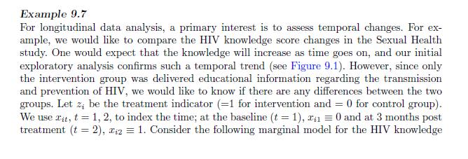
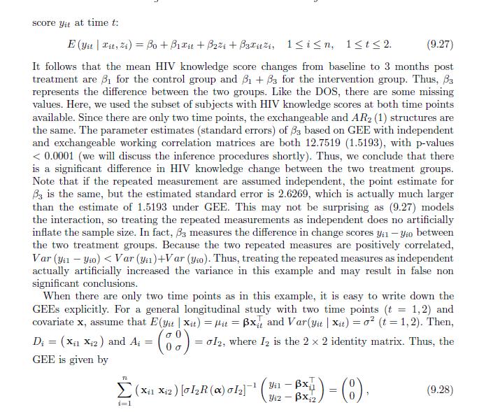
Construct a generalized linear mixed-effects model for the Sexual Health study data with the fixed-effects component similar to that in Example9.7 and random slopes of the time effect and assess the model fit. Example 9.7 For longitudinal data analysis, a primary interest is to assess temporal
Assess the models in Problems 9.12 and 9.14Problem 9.12 is:and Problem 9.14 is:. 9.12 Generalize the model considered in Example 4.11 to a marginal model for the longi- tudinal DOS data and compare the findings with that in Example 4.11.
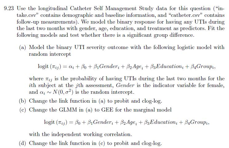
Use the longitudinal Catheter Self Management Study data for this question ("intake.csv" contains demographic and baseline information, and "catheter.csv" contains follow-up measurements). We model the binary response for having any UTIs during the last two months with gender, age, education, and
In this question, we change the response in Problem9.23 to a three-level response by grouping the counts of UTIs into three levels, 0,1 , and \(\geq 2\). Fit the following models and test whether there is a significant group difference.(a) Model the ordinal three-level UTI count outcome with the
Show that for a binary diagnostic test, \(\mathrm{AUC}=\frac{1}{2}\) (sensitivity + specificity).
Show that the ROC curve is invariant under monotone transformation of the test variable.
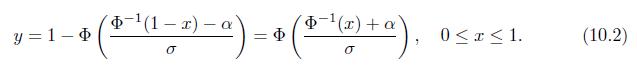
Verify (10.1) and (10.2). Se(c) = 1- $ (c-a) = and Sp(c) (c), cR, (10.1)
Let \(S\) be a curve in the two-dimensional \(x-y\) plane defined parametrically by \(x=F(t)\) and \(y=G(t)\), where \(F\) and \(G\) are smooth functions. Show that the slope of the tangent line at an interior point \(t_{0}\) of \(S\) is \(G^{\prime}\left(t_{0}\right) /
Show that a binormal ROC curve is improper if the two normal distributions for diseased and nondiseased have different variances.
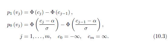
Show that for the binormal model in (10.3), if properness is further assumed, then this model reduces to the cumulative probit model with the disease status as the predictor and the ordinal test result as the response. P1 (v) (c) (cj-1), === cj - - Po (u) = $( a) - $ (c-1-a), j=1,...,m, co =
Let \(t_{k}\) be the test outcome for the diseased \((k=1)\) and nondiseased \((k=0)\) subject. Show(a) \(\mathrm{AUC}=\operatorname{Pr}\left(t_{1} \geq t_{0}\right)\) if \(t_{k}\) is continuous;(b) \(\mathrm{AUC}=\operatorname{Pr}\left(t_{1}>t_{0}\right)+\frac{1}{2}
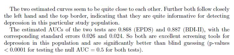
Express the AUC of a binormal ROC curve in terms of the means and variances of the two underlying normal distributions.
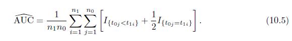
Show that the estimate in (10.5) equals the area under the empirical ROC curve. n1 no AUC = nino I{toj
In assessing the accuracy of HAM-D for the DOS, treat the SCID diagnosis of depression as a gold standard to(a) Estimate the ROC curve;(b) Estimate the AUC;(c) Which cut-points would you suggest based on the data?The ROC and AUC curve Estimate: Sensitivity 0.00 0.25 0.50 0.75 1.00 0.00 0.25 0.50
For the DOS, we would like to manually calculate two two-category NRIs when medical burden is added to HAM-D in the prediction of depression, usinga) 0.5 andb) the sample depression rate as the cut-point. For each cut-point, answer the following questions:(a) Generate the
Verify (10.7) and show(a) \(C_{b} \leq 1\);(b) \(ho_{C C C}=ho_{\text {Pearson }}\), if and only if \(\mu_{1}=\mu_{2}\) and \(\sigma_{1}=\sigma_{2}\).
For the Sexual Health pilot study, compute CCC and ICC between the diary and retrospective recall outcomes for the number of instances of unprotected vaginal sex.
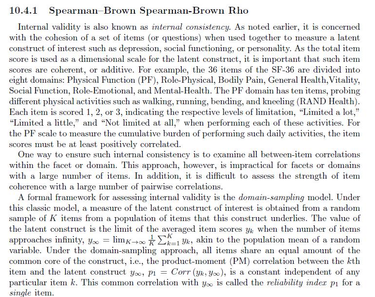
For the domain sampling model described in Section10.4.1, show(a) \(p_{1}=\sqrt{\bar{ho}_{\infty}}\);(b) \(p_{K}=\sqrt{\frac{K \bar{ho}_{\infty}}{1+(K-1) \bar{ho}_{\infty}}}+o(1)\), where \(o(1)\) is a higher order term with \(o(1) \rightarrow 0\) as \(K \rightarrow \infty\). 10.4.1 Spearman-Brown
For the domain sampling model described in Section10.4.1, show(a) If \(\operatorname{Var}\left(y_{k}\right)=\sigma^{2}\) is a constant, the Spearman-Brown \(ho_{K}\) and Cronbach coefficient alpha \(\alpha_{K}\) are identical;(b) If \(\operatorname{Cov}\left(y_{k}, y_{l}\right) \geq c>0\) for
Show that CCC ranges between -1 and 1 and identify the scenarios in which CCC takes the value \(1,-1\), and or 0 .
Show that the moment-based estimate \(\widehat{ho}_{C C C}\) in (10.8) is consistent. pccc = 2812 s+s+ (1.2.) (10.8)
Let \(y_{i k}\) be a continuous outcome for the \(k\) th instrument from the \(i\) th subject \((1 \leq i \leq\) \(n, 1 \leq k \leq K)\). Assume that \(y_{i k}\) follows the LMM in (10.11). Let \(y_{i \infty}=\mu+\lambda_{i}\). Show(a) \(ho_{I C C}=ho_{1}=\operatorname{Corr}\left(y_{i k}, y_{i
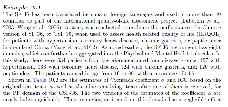
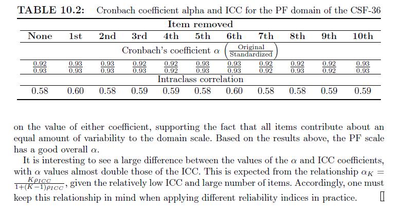
Estimate the reliability index and the Cronbach coefficient alpha for each of the eight domains of CSF-36 based on the study described in Example10.4. Assess whether each item is coherently associated with the other remaining items. Example10.4 Example 10.4 The SF-36 has been translated into many
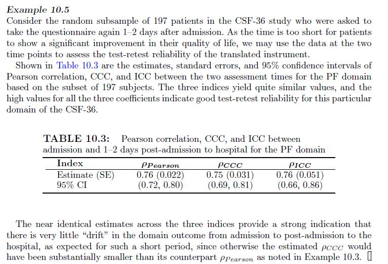
Assess the test-retest reliability for each of the domains of CSF-36 based on the study described in Example10.5. Example 10.5 Consider the random subsample of 197 patients in the CSF-36 study who were asked to take the questionnaire again 1-2 days after admission. As the time is too short for
Suppose for an i.i.d. sample of size \(n\), the disease status, \(d_{i}\), is MCAR with the probability of each \(d_{i}\) being observed given by \(\pi=0.75\).(a) Show that \(\frac{1}{n} \sum_{d_{i} \text { observed }} \frac{d_{i}}{\pi}\) is a consistent estimate of population prevalence,
For the Sexual Health study, check whether the missingness of three-month posttreatment HIV knowledge is MCAR.
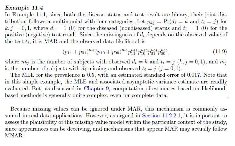
For Example 11.4, we are interested in the sensitivity and specificity of the test.(a) Compute the MLEs of sensitivity and specificity and their asymptotic variances based on the likelihood (11.9).(b) Another way to parametrize the distribution is to use \(\operatorname{Pr}(t=1),
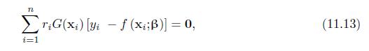
Prove that the estimating equations in (11.13) are unbiased under MCAR, but are generally biased without the stringent MCAR assumption. (x) [y - f (xt;)] = 0, i=1 (11.13)
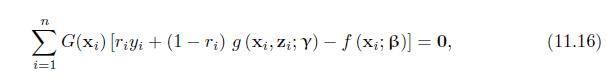
Show that the estimating equations (11.16) are unbiased. IM- G(xi) [Tiyi (1-ri) g (xi, Zi; Y) - f (xi; B)] = 0, (11.16) i=1
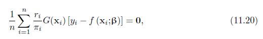
Prove that the estimating equations (11.20) are unbiased. 17 n n i i=1 G(xi) [yi- f (xi;)] = 0, (11.20)
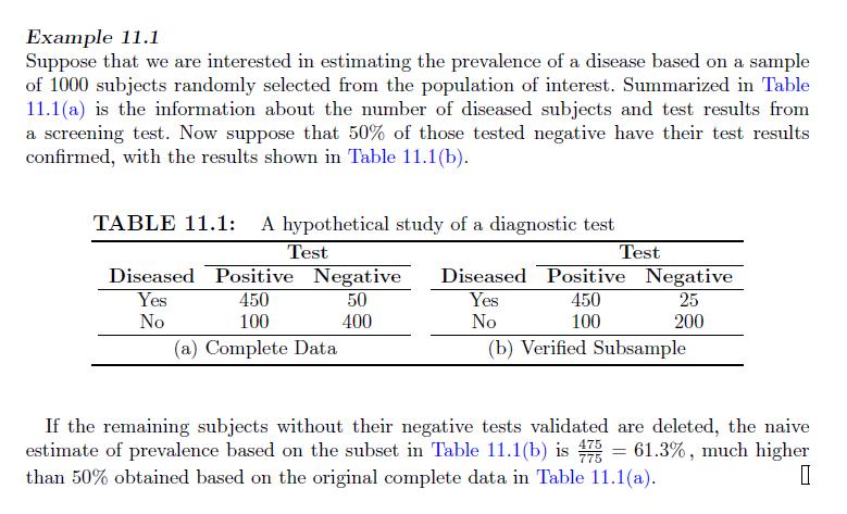
Use mean score, IPW, and MI methods to estimate the sensitivity and specificity of the test in Example 11.1. Example 11.1 Suppose that we are interested in estimating the prevalence of a disease based on a sample of 1000 subjects randomly selected from the population of interest. Summarized in
Use the simulated DOS baseline data (with missing values in depression diagnosis) to assess the accuracy of HAM-D in diagnosis of depression.(a) Estimate the ROC curve using mean score, IPW, and MI methods.(b) Estimate the AUC based on the empirical ROC curve obtained in(a) for each of the mean
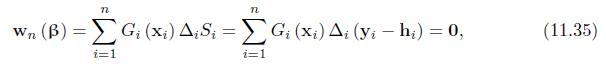
Show that the estimating equations in (11.35) are unbiased. Wn n n (B) = Gi (xi) AiSi = Gi (xi) Ai (yi - h) = 0, i=1 i=1 (11.35)
Prove (11.32) . E (Yi,k | Zi = 0, = e) = E (Yi,k | i = 1, = e) = E (Yi,k | Ti = e), k = 1,2. (11.32)
to the original three-level scale and compare the results from the two versions of the depression diagnosis variable.
For a simple random sample from a population of size \(N\), the subjects are not sampled independently because of the finite size of the population.(a) Show that the probability of being sampled for each subject is \(\frac{n}{N}\), where \(n\) is the number of subjects in the sample.(b) If sampled
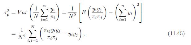
Compute the variance of \(\widehat{\mu}\) in (11.45) via the following steps.(a) Suppose the \(N\) subjects of the population are labeled from 1 to \(N\). The \(i\) th subject with outcome \(y_{i}\) is sampled with the probability \(\pi_{i}\). Show that \(\widehat{\mu}=\frac{1}{N} \sum_{i=1}^{N}
In a study to determine the distribution of time to the occurrence of cancer after exposure to certain type of carcinogen, a group of mice is injected with the carcinogen, and then sacrificed and autopsied after a period of time to see whether cancer cells have been developed. Define the event of
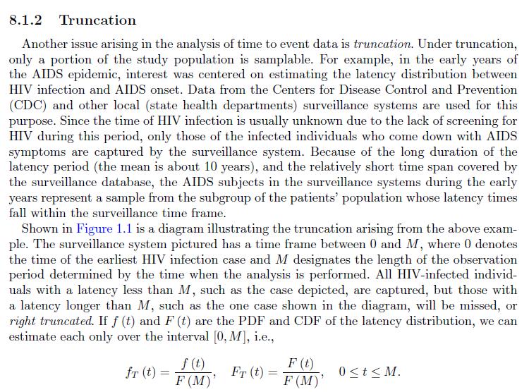
Under the race set up in Section8.1.2, think a scenario when you may have left truncation issue. 8.1.2 Truncation Another issue arising in the analysis of time to event data is truncation. Under truncation, only a portion of the study population is samplable. For example, in the early years of the
Given that a subject survives up to and including time \(t\), how likely is the failure to occur within the next infinitesimal time interval \((t, t+\Delta t)\) ?
For a continuously differentiable survival function \(S(t)\), the hazard function is defined as \(h(t)=-\frac{S^{\prime}(t)}{S(t)}\). Prove that \(S(t)=\exp \left(-\int_{0}^{t} h(s) d s\right)\).
For \(T \sim\) exponential \((\lambda)\), the conditional distribution of \(T-t_{0}\), given \(T \geq t_{0}\), again follows an exponential \((\lambda)\) distribution.
Plot the survival and hazard function for the exponential and Weibull survival times using different parameters and check their shapes.
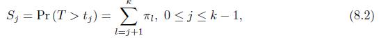
Let \(\left\{\pi_{j}\right\}_{j=1}^{k-1},\left\{S_{j}\right\}_{j=1}^{k-1}\), and \(\left\{p_{j}\right\}_{j=1}^{k-1}\) be defined in (8.1), (8.2), and (8.3). Show that any one of them determines the other two. k = (1,..., ), ; = 1. (8.1) j=1
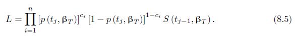
Derive the likelihood (8.5) based on (8.4). L= n Ip(ti, Br)] [1p (tj, r)] S (tj1, r). i=1 (8.5)
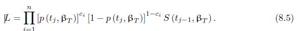
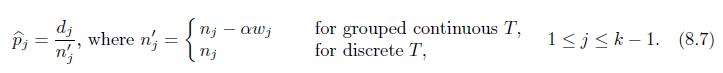
Prove that (8.7) provides the ML estimates based on the likelihood (8.5) and (8.6). n \L = [ [ [p (tj, )]^* [1 p (tj, r)]ci S (tj1, T). (8.5) i=1
For the DOS, we are interested in the time to drop out of the study.(a) Create a life table including the number of subjects at risk, the number of failures (new depression), the number of survivors, and the number of the censored subjects for each gender, at each year;(b) Create a life table
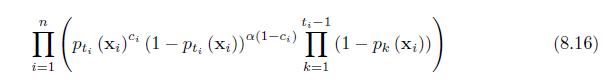
Verify the likelihood (8.16). n t-1 II (Pt, (xi) i (1 Pt, (x;))(1-cs) II (1 Pk (xi)) - (8.16) i=1 k=1
Let \(h_{0}(t)\) denote the hazard function when \(\mathbf{x}_{i}=\mathbf{0}\), and \(S_{0}(t)=\exp \left(\int_{0}^{t} h_{0}(u) d u\right)\) be the corresponding survival function. If \(h\left(t, \mathbf{x}_{i}\right)=\phi\left(\mathbf{x}_{i} ; \boldsymbol{\beta}\right) h_{0}(t)\), show \(S\left(t,
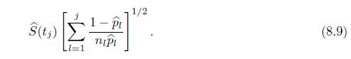
Use the delta method to prove (8.9). (tj) l=1 1-Pi nipi 1/2 (8.9)
Assume that a survival time \(T\) has a constant hazard \(\lambda\) over time interval \(\left[\tau_{j}, \tau_{j+1}\right)\) with \(\log \lambda=\mathbf{x}^{\top} \boldsymbol{\beta}\). Prove \(1-p=\exp \left(-\exp \left(\mathbf{x}^{\top} \boldsymbol{\beta}\right)\right)\), where
Fit the following models for genuinely discrete time to drop-out with age and gender as covariates for the DOS:(a) the proportional hazards models;(b) the proportional odds models.
Check that if \(p_{j}\left(\mathbf{x}_{i}\right)\) is small, then \(\frac{p_{j}\left(\mathbf{x}_{i}\right)}{1-p_{j}\left(\mathbf{x}_{i}\right)} \approx p_{j}\left(\mathbf{x}_{i}\right)\) and hence (8.17) implies \(p_{j}\left(\mathbf{x}_{i}\right) \approx\) \(\phi\left(\mathbf{x}_{i} ;
For the Catheter Study, the patients were assessed bimonthly and the measurements about UTIs, catheter blockages, and replacements cover the previous two months. Thus, the patients were under observation the whole time while they were in the study. So, we can study the survival times from the
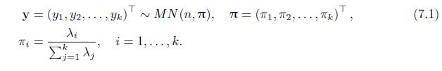
Prove (7.1) . y = (Y1, Y2,Yk) ~ MN (n,), i = 1, MN (n,), = (1, 2,..., k), (7.1) k. "
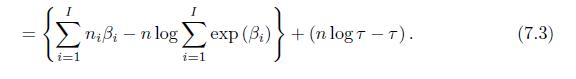
Show that the log-likelihood function in (7.3) can be maximized by maximizing the first term as a function of \(\beta\) and the second term as a function of \(\tau\) separately, and find the MLE of \(\tau\). = i=1 nii-n log i=1 exp (B)+(nlog T-T). (7.3)
Suppose that \(\left\{\mu_{i j}\right\}\) satisfy a multiplicative model\[\begin{equation*}\mu_{i j}=\mu \alpha_{i} \beta_{j}, \quad 1 \leq i \leq I, 1 \leq j \leq J \tag{7.30}\end{equation*}\]where \(\left\{\alpha_{i}, i=1, \ldots, I\right\}\) and \(\left\{\beta_{j}, j=1, \ldots, J\right\}\) are
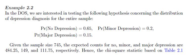
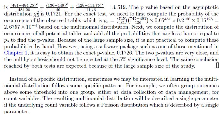
Use loglinear models to test the hypothesis concerning the distribution of depression diagnosis in Example2.2. Example 2.2 In the DOS, we are interested in testing the following hypothesis concerning the distribution of depression diagnosis for the entire sample: Pr(No Depression) = 0.65, Pr(Minor
For the DOS, use the three-level depression diagnosis and variable MS for marital status as defined in Section 4.2.2 to test for uniform association, assuming that both the depression diagnosis and MS are ordered according their defined values.
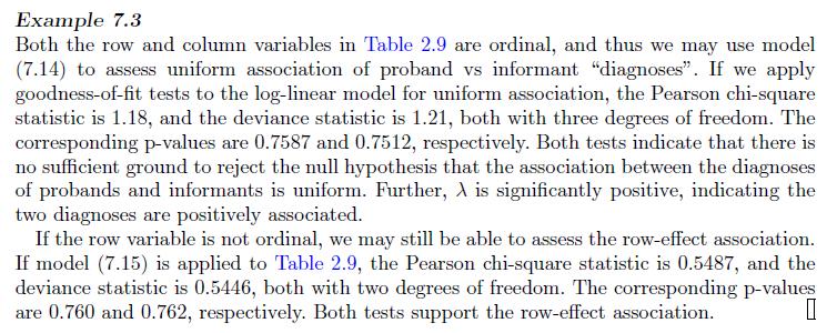
In Example 7.3, we assessed the uniform association between the diagnosis of probands and informants. Perform the following alternative approaches for assessing uniform association and compare the results with that of Example 7.3(a) Fit a saturated log-linear model and test whether the association
Prove that model (7.15) is indeed the model for the row-effect association. log (ij) = ++iy, 1iI,1 j J. (7.15)
For the DOS, use the three-level depression diagnosis and variable MS for marital status as defined in Section4.2.2. If MS is not ordered, we may not be able to talk about the uniform association. However, we may assess MS-effect association, the roweffect association when MS is treated as the row
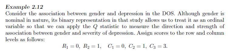
Redo Example 2.12 using log-linear models. Example 2.12 Consider the association between gender and depression in the DOS. Although gender is nominal in nature, its binary representation in that study allows us to treat it as an ordinal variable so that we can apply the Q statistic to measure the
Each of the three random variables \(x, y\), and \(z\) has two levels: 0 and 1 . The joint distribution of these three variables can be determined from the facts \(\operatorname{Pr}(x=0, y=\) \(0, z=0)=\frac{1}{4}, \operatorname{Pr}(x=0, y=1, z=1)=\frac{1}{4}, \operatorname{Pr}(x=1, y=0,
Prove that under the mutual independence log-linear model (7.19), the three variables are indeed mutually independent. log ijk = logy + log i+++ log+j+ + log ++k = X + X + X + X. (7.19)
Prove that three variables being mutually independent implies that any two of them are marginally independent, conditionally independent, and any one of them is jointly independent with the others.
Prove that if \(x\) is jointly independent with \(y\) and \(z\), then \(x\) and \(y\) are marginally independent.
Prove that if \(x\) is jointly independent with \(y\) and \(z\), then \(x\) and \(y\) are conditionally independent.
To obtain the log-linear models for association homogeneity, we need the following two key facts:(a) Prove (7.25).(b) Prove that \(\lambda_{i^{\prime} j k}^{x y z}+\lambda_{i j^{\prime} k}^{x y z}=\lambda_{i j k}^{x y z}+\lambda_{i^{\prime} j^{\prime} k}^{x y z}\) for all \(i, i^{\prime}, j,
Verify that under the mutual independent log-linear model (7.23), the variable \(y\) is independent with the other two. log ijk = log +logi+k+log +j+ = X + X + x + X + X (7.23)
Verify the numbers of free parameters in the model (7.17). log ij+i+j+Aij, all i, j, (7.17)
Write down the log-linear model for quasi-symmetry, and count the number of free parameters in the model.
Prove under the paradigm of a multinomial distribution that if \(x\) and \(y\) are homogeneously associated, then \(y\) and \(z\) as well as \(x\) and \(z\) are also homogeneously associated.
Prove that \(\exp \left(\lambda_{111}^{x y z}\right)=\frac{\pi_{2,2,2} / \pi_{1,2,2}}{\pi_{2,1,2} / \pi_{1,1,2}} / \frac{\pi_{2,2,1} / \pi_{1,2,1}}{\pi_{2,1,1} / \pi_{1,1,1}}\) for a \(2 \times 2 \times 2\) three-way table.
For the DOS, use the three-level depression diagnosis.(a) Use the Poisson log-linear model to test whether depression and gender are independent.(b) Use methods for contingency tables studied in Chapter 2 to test the independency between depression and gender.(c) Compare parts (a) and (b), and
For the DOS, use the three-level depression diagnosis and variable MS for marital status as defined(a) whether depression, gender, and MS are mutually independent;(b) whether depression is independent of MS given gender;(c) whether depression is jointly independent of gender and MS.
Use the log-linear model to test whether SCID (two levels: no depression and depressed including major and minor depression) and dichotomized EPDS (EPDS \(\leq 9\) and EPDS \(>9)\) are homogeneously associated across the three age groups in the PPD.
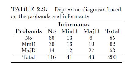
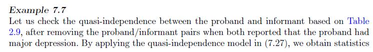
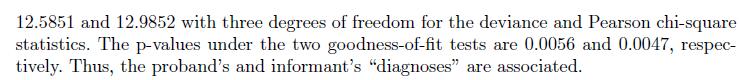
Check that for Example 7.7, you may obtain different (incorrect) results if the random zero is removed from the data set for data analysis. Example 7.7 Let us check the quasi-independence between the proband and informant based on Table 2.9, after removing the proband/informant pairs when both
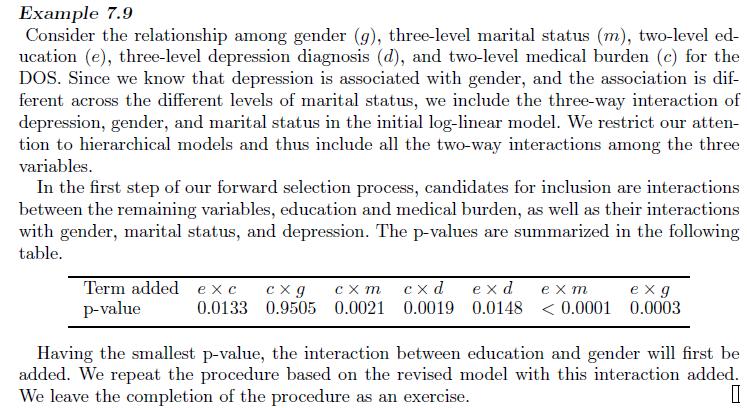
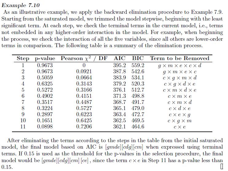
Complete the forward model selection in Example7.9 and compare it with the models selected in Examples7.10 Example 7.9 Consider the relationship among gender (g), three-level marital status (m), two-level ed- ucation (e), three-level depression diagnosis (d), and two-level medical burden (c) for
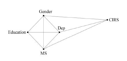
Check that [edgm \(][\) cdgm \(]\) is a graphical model. Education Gender MS Dep CIRS
Check that there are at least \(2\left(\begin{array}{c}n \\ 3\end{array}\right)\) different hierarchical models which contain all twoway interaction terms for an \(n\)-way contingency table.
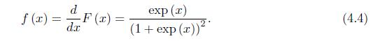
Consider a random variable \(x\) following the standard logistic distribution with the \(\mathrm{CDF}\) and PDF given in (4.3) and (4.4).(a) Show that the PDF in (4.4) is symmetric about 0.(b) Show that CDF in (4.3) is strictly increasing on \((-\infty, \infty)\).(c) Plot the CDF in (4.3) and
Prove that if\[\operatorname{logit}\left(\operatorname{Pr}\left(y_{i}=1 \mid \mathbf{x}_{i}\right)\right)=\beta_{0}+\mathbf{x}^{\top} \boldsymbol{\beta}\]and\[\operatorname{logit}\left(\operatorname{Pr}\left(y_{i}=0 \mid \mathbf{x}_{i}\right)\right)=\alpha_{0}+\mathbf{x}^{\top}
If \(\Sigma\) is an \(n \times n\) invertible matrix and \(K\) is a \(k \times n\) matrix with \(\operatorname{rank} k(k \leq n)\), show that \(K \Sigma K^{\top}\) is invertible.
Show that the Wald statistic in (4.15) does not depend on the specific equations used. Specifically, suppose that \(K\) and \(K^{\prime}\) are two equivalent systems of equations for a linear hypothesis, i.e., the row spaces generated by the rows of the two matrices are the same, then the
Use a logistic model to assess the relationship between CIRSD and Depd, with Depd as the outcome variable.(a) Write down the logistic model.(b) Write down the null hypothesis that CIRSD has no effect.(c) Write down the null hypothesis that there is no difference between CIRSD \(=1\) and CIRSD
Based on a logistic regression of Depd on some covariates, we obtained the following prediction equation:\[\begin{align*}\operatorname{logit}[\widehat{\operatorname{Pr}}(D e p d=1)] & =1.13-0.02 \text { Age }-1.52 M S D+0.29 R 1+0.06 R 2 \\& +0.90 M S D * R 1+1.79 M S D * R 2
In suicide studies, alcohol use is found to be an important predictor of suicide ideation. Suppose the following logistic model is used to model the effect:\[\begin{equation*}\operatorname{logit}[\operatorname{Pr}(\text { has suicide ideation })]=\beta_{0}+\beta_{1} * \operatorname{Drink}
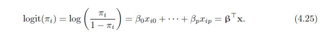
Consider the logistic regression in (4.25). Show that for each \(j(1 \leq j \leq p), T_{j}(x)=\) \(\sum_{i=1}^{n} y_{i} x_{i j}\) is a sufficient statistic for \(\beta_{j}\). logit (T) = log 1 i ) == Boxio + + Bpxip=Bx. (4.25)
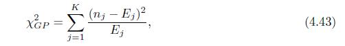
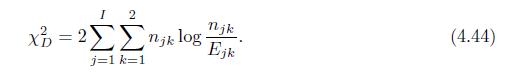
Use the fact that \(x \log x=(x-1)+(x-1)^{2} / 2+o\left((x-1)^{2}\right)\) to show that the deviance test statistic \(D^{2}\) in (4.43) has the same asymptotic distribution as the general Pearson chi-square statistic in (4.44). XGP = K j=1 (n; - Ej) Ej (4.43)
For the DOS, we are interested in how MS and gender are related with the depression outcome. Based on the logistic model: Dep \(\sim\) MS | Gender (MS, Gender, and their interaction), answer the following questions:(a) Test the goodness of fit of the model.(b) Is the interaction significant?(c)
We add age as a continuous covariate to the model in the last problem and consider the logistic model: Dep \(\sim\) MS+ Gender+Age.(a) Test the goodness of fit of the model.(b) Use Box-Tidwell test to test the linearity assumption for Age.(c) Apply Pregibon's link test to the model.

Showing 1500 - 1600 of 1977

First
6
7
8
9
10
11
12
13
14
15
16
17
18
19
20

Step by Step Answers

Services

Sitemap
Fun
Definitions
Become Tutor
Used Textbooks
Study Help Categories
Recent Questions
Expert Questions
Campus Wear
Sell Your Books

Company Info

Security
Copyrights
Privacy Policy
Terms & Conditions
SolutionInn Fee
Scholarship
Online Quiz
Give Feedback, Get Rewards

Get In Touch

About Us
Contact Us
Career
Jobs
FAQ
Student Discount
Campus Ambassador

Secure Payment

Download Our App

© 2026 SolutionInn. All Rights Reserved