New Semester Started Get 50% OFF Study Help! --h --m --s Claim Now

Question Answers

Textbooks

Find textbooks, questions and answers

Oops, something went wrong!

Change your search query and then try again

Result Not Found

Books FREE
Study Help
Tutors
AI Study Planner NEW
Sell Books

Search
Sign In
Register

study help
statistics
elementary statistics in social research

Elementary Statistics Picturing The World 7th Global Edition Betsy Farber, Ron Larson - Solutions

Based on the results of a life-testing experiment, a manufacturer says there is a 0.07 probability that a randomly chosen component will last for 3 hours.Classify the statement as an example of classical probability, empirical probability, or subjective probability. Explain your reasoning.
The probability of randomly selecting an ace from a standard deck of 52 playing cards is about 0.077.Classify the statement as an example of classical probability, empirical probability, or subjective probability. Explain your reasoning.
The chance that it will rain tomorrow is 25%.Classify the statement as an example of classical probability, empirical probability, or subjective probability. Explain your reasoning.
The probability that a person will be able to swim 20 miles is 40%.Classify the statement as an example of classical probability, empirical probability, or subjective probability. Explain your reasoning.
The probability of getting a sum of 10 or 11 when a pair of dice is rolled is 5 36.Classify the statement as an example of classical probability, empirical probability, or subjective probability. Explain your reasoning.
Rolling a die three times, getting two sixes, and rolling it a fourth time and getting a two.Determine whether the events are independent or dependent. Explain your reasoning.
Participating in a training camp for running marathons and successfully completing a marathon run.Determine whether the events are independent or dependent. Explain your reasoning.
Regularly attending the lectures of a course and passing that course.Determine whether the events are independent or dependent. Explain your reasoning.
You are given that P(A) = 0.35 and P(B´) = 0.25. Do you have enough information to find P(B) and P(A and B)? Explain.Determine whether the events are independent or dependent. Explain your reasoning.
Two balls are drawn from a bag containing 20 white and 5 black balls. In the first draw a ball is drawn at random and then replaced in the bag. In the second, a ball is drawn again at random. Find the probability of getting black balls in both the draws. Is this an unusual event? Explain.Determine
A bag has 12 white, 10 red and 8 black balls. What is the probability that without looking in the bag, you will first select and remove a white ball, and then select either a red or black ball? Is this an unusual event? Explain.Determine whether the events are independent or dependent. Explain your
Event A: Randomly select a person who is a professional singer.Event B: Randomly select a person who is a professional dancer Determine whether the events are mutually exclusive. Explain your reasoning.
Event A: Randomly select a U.S. citizen of Indian origin..Event B: Randomly select a U.S. citizen of Chinese origin.Determine whether the events are mutually exclusive. Explain your reasoning.
In a random sample of 300 male professionals it is found that 40% play golf, 60% play soccer and 30% play both golf and soccer. Find the probability that a person selected at random from this sample plays golf or soccer.Find the probability.
In a community 60% of the population speaks English, 30% speaks Spanish and 15% speaks both English and Spanish. Find the probability that a randomly chosen person from this community speaks English or Spanish.Find the probability.
A card is randomly selected from a standard deck of 52 playing cards. Find the probability that the card is between 7 and 10, inclusive, or is black.Find the probability.
A 10-sided die, numbered 1 to 10, is rolled. Find the probability that the roll results in an even number or a number greater than 6.Use the pie chart at the left, which shows the percent distribution of the number of students in U.S. public schools in a recent year.
11P2 Perform the indicated calculation.
7C4 Perform the indicated calculation.
Six different letters are to be put in six envelopes of different colors in a manner that each envelope gets only one letter. In how many ways can this be done?Use combinations and permutations.
A basketball coach has to choose 5 players from a list of 12 players. In how many ways can the coach choose the 5 players?Use combinations and permutations.
In a game of cards you are dealt a hand of six cards at random from a standard deck of 52 cards. You are declared winner if you are being dealt an ace, two kings and three queens. Find the probability of you winning the game.Use counting principles to find the probability.
A code consists of two distinct letters followed by three digits. The last digit cannot be 0 or 1.What is the probability of guessing the security code on the first try?Use counting principles to find the probability.
A batch of 100 mobile phones contains 5 smartphones. What is the probability that a sample of three phones will have(a) no smartphones?(b) all smartphones?(c) at least one smartphone?(d) at least one non-smartphone?Use counting principles to find the probability.
A batch of 200 laptops contains three defective laptops. You choose three laptops at random. What is the probability that you have(a) no defective laptops?(b) all three defective laptops?(c) two defective laptops?(d) at least one defective laptop?Use counting principles to find the probability.
A panel consists of three female and seven male experts. Three experts are chosen at random from this panel to serve in a selection committee. What is the probability of choosing(a) three men?(b) all women?(c) two men and one woman?(d) one man and two women?Use counting principles to find the
The access code for a warehouse’s security system consists of six digits. The first digit cannot be 0 and the last digit must be even. How many access codes are possible?
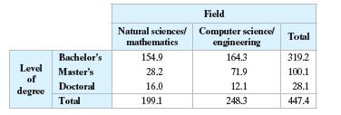
The table shows the numbers (in thousands) of earned degrees by level in two different fields, conferred in the United States in a recent year.A person who earned a degree in the year is randomly selected. Find the probability of selecting someone who(a) earned a bachelor’s degree.(b) earned a
Which event(s) in Exercise 2 can be considered unusual? Explain.Data from Exercises 2The table shows the numbers (in thousands) of earned degrees by level in two different fields, conferred in the United States in a recent year.A person who earned a degree in the year is randomly selected. Find the
Determine whether the events are mutually exclusive. Then determine whether the events are independent or dependent. Explain your reasoning.Event A: A bowler having the highest game in a 40-game tournament Event B: Losing the bowling tournament
From a pool of 30 candidates, the offices of president, vice president, secretary, and treasurer will be filled. In how many different ways can the offices be filled?
A shipment of 250 netbooks contains 3 defective units. Determine how many ways a vending company can buy three of these units and receive(a) no defective units.(b) all defective units.(c) at least one good unit.
In Exercise 6, find the probability of the vending company receiving(a) no defective units.(b) all defective units.(c) at least one good unit.Data from Exercises 6A shipment of 250 netbooks contains 3 defective units. Determine how many ways a vending company can buy three of these units and
Determine whether each random variable x is discrete or continuous. Explain your reasoning.1. Let x represent the number of Fortune 500 companies that lost money in the previous year.2. Let x represent the volume of gasoline in a 21-gallon tank.
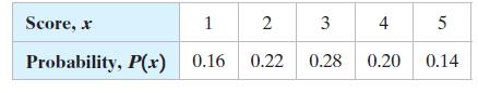
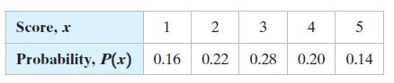
An industrial psychologist administered a personality inventory test for passive-aggressive traits to 150 employees. Each individual was given a whole number score from 1 to 5, where 1 is extremely passive and 5 is extremely aggressive. A score of 3 indicated neither trait. The results are shown at
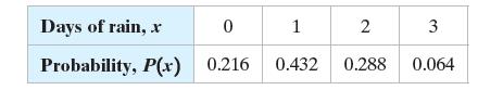
Verify that the distribution for the three-day forecast and the number of days of rain is a probability distribution. Days of rain, x 0 1 2 3 Probability, P(x) 0.216 0.432 0.288 0.064
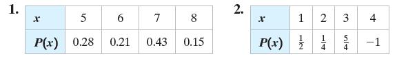
Determine whether each distribution is a probability distribution. Explain your reasoning. 1. x 5 6 7 8 P(x) 0.28 0.21 0.43 0.15 2. x 1 2 P(x) 14 3 51 4 -1
The probability distribution for the personality inventory test for passive aggressive traits discussed in Example 2 is shown below. Find the mean score.Data from Example 2An industrial psychologist administered a personality inventory test for passive-aggressive traits to 150 employees. Each
The probability distribution for the personality inventory test for passiveaggressive traits discussed in Example 2 is shown below. Find the variance and standard deviation of the probability distribution.Data from Example 2An industrial psychologist administered a personality inventory test for
At a raffle, 1500 tickets are sold at \($2\) each for four prizes of \($500,\) \($250,\) \($150,\) and \($75.\) You buy one ticket. Find the expected value and interpret its meaning.
Let x represent the number of times a book is issued from the library.Determine whether the random variable x is discrete or continuous. Explain.
Let x represent the weight of a student’s school bag.Determine whether the random variable x is discrete or continuous. Explain.
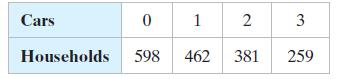
The number of Sedan cars per household in a small town(a) construct a probability distribution,(b) graph the probability distribution using a histogram and describe its shape. Cars 0 1 2 3 381 259 Households 598 462
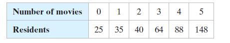
The number of movies watched by the residents of a locality per week(a) construct a probability distribution,(b) graph the probability distribution using a histogram and describe its shape. Number of movies Residents 0 1 2 3 4 5 25 35 40 40 64 88 148 88
Use the probability distribution you made in Exercise 19 to find the probability of randomly selecting a household that has(a) one or two cars,(b) less than two cars,(c) between one and three cars, inclusive, and(d) at least two cars.Data from Exercises 19The number of Sedan cars per household in a
Use the probability distribution you made in Exercise 20 to find the probability of randomly selecting a resident of the locality who watches(a) two or three movies,(b) more than three movies,(c) between one and four movies, inclusive,(d) between two and five movies, inclusive, and(d) at most three
In Exercise 19, would it be unusual for a household to have three Sedan cars? Explain your reasoning.Data from Exercises 19The number of Sedan cars per household in a small town Cars 0 1 2 3 381 259 Households 598 462
In Exercise 20, would it be unusual for a resident to not watch any movie in a week at all? Explain your reasoning.Data from Exercises 20The number of movies watched by the residents of a locality per week Number of movies Residents 0 1 2 3 4 5 25 35 40 40 64 88 148 88
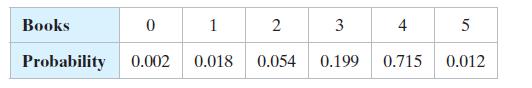
The number of books per shelf in a library(a) find the mean, variance, and standard deviation of the probability distribution,(b) interpret the results. Books 0 1 2 3 4 5 Probability 0.002 0.018 0.054 0.199 0.715 0.012
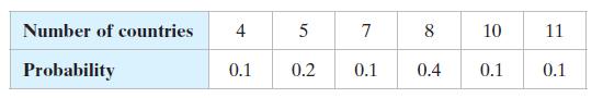
The number of countries who played Women’s Cricket World Cup from 1973 through 2013(a) find the mean, variance, and standard deviation of the probability distribution,(b) interpret the results. Number of countries 4 5 7 8 $ 10 911 Probability 0.1 0.2 0.1 0.4 0.1 0.1
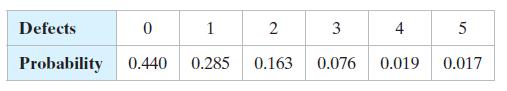
The number of defects per 1000 LED lamps inspected(a) find the mean, variance, and standard deviation of the probability distribution,(b) interpret the results. Defects 0 1 2 3 4 5 Probability 0.440 0.285 0.163 0.076 0.019 0.017
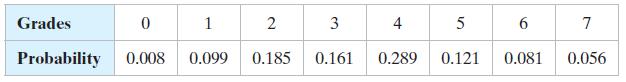
The number of A grades received in different subjects per student(a) find the mean, variance, and standard deviation of the probability distribution,(b) interpret the results. Grades 0 1 2 3 4 5 6 7 Probability 0.008 0.099 0.185 0.161 0.289 0.121 0.081 0.056
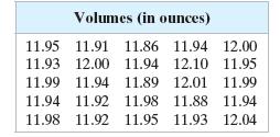
Construct a frequency histogram for the data set using seven classes.Use the data set shown in the table at the left, which represents the actual liquid volumes (in ounces) in 25 twelve-ounce cans. Volumes (in ounces) 11.95 11.91 11.86 11.94 12.00 11.93 12.00 11.94 12.10 11.95 11.99 11.94 11.89
Construct a relative frequency histogram for the data set using seven classes.Use the data set shown in the table at the left, which represents the actual liquid volumes (in ounces) in 25 twelve-ounce cans. Volumes (in ounces) 11.95 11.91 11.86 11.94 12.00 11.93 12.00 11.94 12.10 11.95 11.99 11.94
Use a stem-and-leaf plot to display the data set. Describe any patterns.Use the data set, which represents the pollution indices for 24 U.S. cities. 22 41 46 50 38 57 65 49 41 23 38 65 28 36 63 54 33 28 53 32 39 43 56 39
Use a dot plot to display the data set. Describe any patterns.Use the data set, which represents the pollution indices for 24 U.S. cities. 22 41 46 50 38 57 65 49 41 23 38 65 28 36 63 54 33 28 53 32 39 43 56 39
Six test scores are shown below. The first 4 test scores are 15% of the final grade, and the last two test scores are 20% of the final grade. Find the weighted mean of the test scores.80 70 84 93 89 78
The weights (in lbs) of 14 newborn babies.Find the range, mean, variance, and standard deviation of the population data set. 7 5 12 12 6 9 11 4 7 6 8 7 10 9
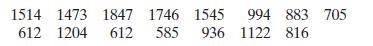
The insurance claims (in dollars) from an auto insurance company.Find the range, mean, variance, and standard deviation of the sample data set. 1514 1473 1847 1746 1545 612 1204 612 585 994 883 705 936 1122 816
Annual household expenditures (in dollars) of a random sample of university professors:Find the range, mean, variance, and standard deviation of the sample data set. 37,224 40,964 43,724 36,188 38,882 38,157 39,914 37,443.
The mean wages for a sample of employees in a company was \($18.00\) per day with a standard deviation of \($2.50\) per day. Between what two values do 95% of the data lie? (Assume the data set has a bell-shaped distribution.)Use the Empirical Rule.
The mean wages for a sample of employees in a company was \($16.50\) per day with a standard deviation of \($1.50\) per month. Estimate the percent of wages between \($12.00\) and \($21.00\) per day. (Assume the data set has a bell-shaped distribution.)Use the Empirical Rule.
In a certain examination, the mean score per student for 20 students is 75 with a standard deviation of 8.5. Using Chebychev’s Theorem, determine at least how many of the students scored between 58 and 92.
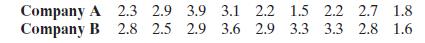
Sample dividends (in %) paid by two companies are listed:Find the coefficient of variation for each of the two data sets. Then compare the results. Company A 2.3 2.9 3.9 Company B 2.8 2.5 2.9 3.1 2.2 1.5 2.2 2.7 1.8 3.6 2.9 3.3 3.3 2.8 1.6
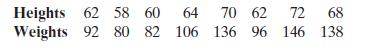
The heights (in inches) and weights (in lbs) of 8 students in a secondary school are listed.Find the coefficient of variation for each of the two data sets. Then compare the results. Heights 62 58 60 Weights 92 80 82 64 70 62 72 68 106 136 96 146 138
A worker’s income of \($32\) represents the 15th percentile of the incomes. What percentage of workers earns more than \($32\)?
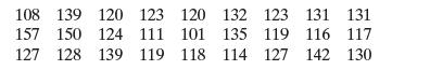
The data set represents the numbers of minutes a sample of 27 people exercise each week.(a) Construct a frequency distribution for the data set using five classes. Include class limits, midpoints, boundaries, frequencies, relative frequencies, and cumulative frequencies.(b) Display the data using a
Use frequency distribution formulas to approximate the sample mean and the sample standard deviation of the data set in Exercise 1.Data from Exercise 1The data set represents the numbers of minutes a sample of 27 people exercise each week. 108 139 120 123 120 132 123 131 131. 157 150 124 111 127
The elements with known properties can be classified as metals (57 elements), metalloids (7 elements), halogens (5 elements), noble gases (6 elements), rare earth elements (30 elements), and other nonmetals (7 elements). Display the data using(a) a pie chart(b) a Pareto chart.
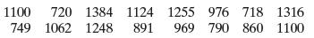
Weekly salaries (in dollars) for a sample of construction workers are listed.(a) Find the mean, median, and mode of the salaries. Which best describes a typical salary?(b) Find the range, variance, and standard deviation of the data set.(c) Find the coefficient of variation of the data set. 1100
The mean price of new homes from a sample of houses is \($180,000\) with a standard deviation of \($15,000\). The data set has a bell-shaped distribution. Using the Empirical Rule, between what two prices do 95% of the houses fall?
Refer to the sample statistics from Exercise 5 and determine whether any of the house prices below are unusual. Explain your reasoning.(a) $225,000(b) $80,000(c) $200,000(d) $147,000Data from Exercises 5The mean price of new homes from a sample of houses is \($180,000\) with a standard
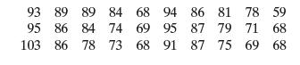
The numbers of regular season wins for each Major League Baseball team in 2016 are listed. Display the data using a box-and-whisker plot. 93 89 89 84 68 94 86 81 78 59 95 86 84 74 69 95 87 79 71 68 103 86 78 73 68 91 87 75 69 68
For quality assurance, every fortieth toothbrush is taken from each of four assembly lines and tested to make sure the bristles stay in the toothbrush.Identify the sampling technique used, and discuss potential sources of bias (if any). Explain.
Using random digit dialing, researchers asked 1090 U.S. adults their level of education.Identify the sampling technique used, and discuss potential sources of bias (if any). Explain.
In 2016, a worldwide study of workplace fraud found that initial detections of fraud resulted from a tip (39.1%), an internal audit (16.5%), management review (13.4%), detection by accident (5.6%), account reconciliation (5.5%), surveillance/monitoring (1.9%), confession (1.3%), or some other means
In 2016, the median annual salary of a marketing account executive was $68,232.Determine whether the number is a parameter or a statistic. Explain your reasoning.
In a survey of 1002 U.S. adults, 88% said that fake news has caused a great deal of confusion or some confusion. Determine whether the number is a parameter or a statistic. Explain your reasoning.
The mean annual salary for a sample of electrical engineers is \($86,500\), with a standard deviation of \($1500\). The data set has a bell-shaped distribution.(a) Use the Empirical Rule to estimate the percent of electrical engineers whose annual salaries are between \($83,500\) and $89,500.(b)
A survey of 339 college and university admissions directors and enrollment officers found that 72% think their institution is losing potential applicants due to concerns about accumulating student loan debt. Identify the population and the sample.
A survey of 67,901 Americans ages 12 years or older found that 1.6% had used pain relievers for nonmedical purposes.Identify the population and the sample.
To study the effect of using digital devices in the classroom on exam performance, researchers divided 726 undergraduate students into three groups, including a group that was allowed to use digital devices, a group that had restricted access to tablets, and a control group that was
In a study of 7847 children in grades 1 through 5, 15.5% have attention deficit hyperactivity disorder.Determine whether the study is an observational study or an experiment. Explain.
The numbers of stolen bases during the 2016 season for Chicago Cubs players who stole at least one base are listed.2 8 3 2 13 12 6 2 1 5 11 1Determine whether the data are qualitative or quantitative, and determine the level of measurement of the data set.
The six top-earning states in 2015 by median household income are listed.1. New Hampshire 2. Alaska 3. Maryland 4. Connecticut 5. Minnesota 6. New Jersey Determine whether the data are qualitative or quantitative, and determine the level of measurement of the data set.
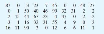
The numbers of tornadoes by state in 2016 are listed.(a) Draw a box-and-whisker plot that represents the data set(b) describe the shape of the distribution. 87 0 3 23 7 45 0 1 50 40 46 99 0 0 48 27 32 31 2 15 44 67 23 4 47 0 3 1 16 32 31 55 4 9 16 11 90 30 12 6 6 11 22231 2201
Five test scores are shown below. The first 4 test scores are 15% of the final grade, and the last test score is 40% of the final grade. Find the weighted mean of the test scores.85 92 84 89 91
Tail lengths (in feet) for a sample of American alligators are listed.(a) Find the mean, median, and mode of the tail lengths. Which best describes a typical American alligator tail length? Explain your reasoning.(b) Find the range, variance, and standard deviation of the data set.
A study shows that life expectancies for Americans have increased or remained stable every year for the past five years.(a) Make an inference based on the results of the study.(b) What is wrong with this type of reasoning?
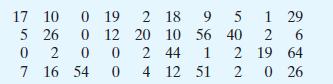
Construct a frequency distribution for the data set using eight classes. Include class limits, midpoints, boundaries, frequencies, relative frequencies, and cumulative frequencies.Use the data set, which represents the points scored by each player on the Montreal Canadiens in the 2015–2016 NHL
Describe the shape of the distribution.Use the data set, which represents the points scored by each player on the Montreal Canadiens in the 2015–2016 NHL season. 7507 17 10 0 19 2 18 9 5 5 26 26 0 12 20 10 56 40 1 29 26 2 00 2 44 12 19 64 16 54 04 12 51 2 0 26
Construct a relative frequency histogram using the frequency distribution in Exercise 17. Then determine which class has the greatest relative frequency and which has the least relative frequency.Use the data set, which represents the points scored by each player on the Montreal Canadiens in the
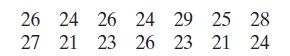
The English scores for a sample of 14 studentsFind the mean, the median, and the mode of the data, if possible. If any measure cannot be found or does not represent the center of the data, explain why. 26 24 26 24 29 25 28 27 21 23 26 23 21 24
The salaries (in thousand dollars) of a sample of 10 employeesFind the mean, the median, and the mode of the data, if possible. If any measure cannot be found or does not represent the center of the data, explain why 225 410 368 310 228 298 361 159 486 296
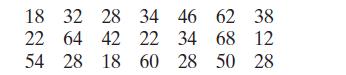
The durations (in minutes) of idle times at a factory in the last 10 monthsFind the mean, the median, and the mode of the data, if possible. If any measure cannot be found or does not represent the center of the data, explain why 18 32 28 22 64 42 54 28 18 34 46 62 38 22 34 68 12 22 60 28 50 28
The ages (in completed years) of the youngest leaders at the time of assuming officeFind the mean, the median, and the mode of the data, if possible. If any measure cannot be found or does not represent the center of the data, explain why. 33 37 37 39 39 41 43 43 44 45
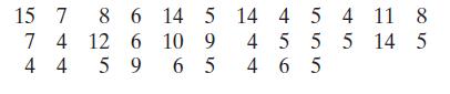
The numbers of weeks the 33 leading movies remained at number 1 as of March 2018.Find the mean, the median, and the mode of the data, if possible. If any measure cannot be found or does not represent the center of the data, explain why. 15 7 8 6 14 5 14 4 5 4 11 8 7 4 4 4 12 6 10 9 4 5 5 5 14 5 59
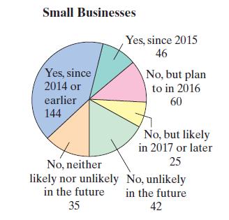
The pie chart at the left shows the responses of a sample of 352 small-business owners who were asked whether their business has a website.Find the mean, the median, and the mode of the data, if possible. If any measure cannot be found or does not represent the center of the data, explain why.
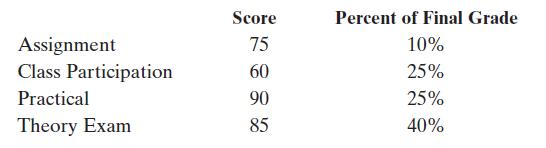
The scores and their percents of the final grade for a biology student are shown below. What is the student’s mean score?Find the weighted mean of the data. Score Percent of Final Grade Assignment 75 10% Class Participation 60 25% Practical 90 25% Theory Exam 85 40%
In Exercise 41, an error was made in grading your practical. Instead of getting 90, you scored 100.What is your new weighted mean?Data from Exercises 41The scores and their percents of the final grade for a biology student are shown below. What is the student’s mean score?Find the weighted mean

Showing 1200 - 1300 of 1977

First
6
7
8
9
10
11
12
13
14
15
16
17
18
19
20

Step by Step Answers

Services

Sitemap
Fun
Definitions
Become Tutor
Used Textbooks
Study Help Categories
Recent Questions
Expert Questions
Campus Wear
Sell Your Books

Company Info

Security
Copyrights
Privacy Policy
Terms & Conditions
SolutionInn Fee
Scholarship
Online Quiz
Give Feedback, Get Rewards

Get In Touch

About Us
Contact Us
Career
Jobs
FAQ
Student Discount
Campus Ambassador

Secure Payment

Download Our App

© 2026 SolutionInn. All Rights Reserved