New Semester Started Get 50% OFF Study Help! --h --m --s Claim Now

Question Answers

Textbooks

Find textbooks, questions and answers

Oops, something went wrong!

Change your search query and then try again

Result Not Found

Books FREE
Study Help
Tutors
AI Study Planner NEW
Sell Books

Search
Sign In
Register

study help
mathematics
statistics

Understanding Business Statistics 1st edition Stacey Jones, Tim Bergquist, Ned Freed - Solutions

Refer to Exercise 5 (consumer confidence), where the least squares line is ŷ = 162 - 12x. a. Report the SSE and sy.x values. b. Tell what these measures represent.
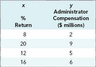
Refer to Exercise 8 (hedge fund returns and administrator compensation), where the least squares line is ŷ = 2.2 .55x. a. Report the SSE and syx values. b. One of the properties of the least squares line is that it minimizes SSE and syx - two measures of error. Suppose instead of
Refer to Exercise 9 (customer wait time), where the least squares line is ŷ = 126 1.8x.a. Report the SSE and s y. x values.b. Tell what these measures represent
In a recent study, simple linear regression was used to link the annual R & D budget of various high tech companies to the number of patents obtained by company researchers. Data for the four companies that participated in the study are shown below.a. Show the data in a scatter diagram and use
Refer to Exercise 10 (too much information), where the least squares line is ŷ66 6.8x. a. Report the SSE and s y. x values.b. Tell what these measures represent.
Compute and interpret the r2 and r values for the regression analysis described in Exercise 1 (Jessica’s coffee shop). Be sure to show the correct sign for r.
Compute and interpret the r2 and r values for the regression analysis described in Exercise 2 (R & D budget).
Compute and interpret the r2 and r values for the regression analysis described in Exercise 3 (interest rates and home sales).
Compute and interpret the r2 and r values for the regression analysis described in Exercise 4 (employee turnover).
Compute and interpret the r2 and r values for the regression analysis described in Exercise 5 (consumer confidence index). (To speed your calculations: SST 2000 and SSR 1440.)
Compute and interpret the r2 and r values for the regression analysis described in Exercise 6 (Amazon sales). (To speed your calculations: SST 320 and SSR 160.)
Compute and interpret the r2 and r values for the regression analysis described in Exercise 8 (Hedge fund compensation). (To speed your calculations: SST 25 and SSE .8.)
Compute and interpret the r2 and r values for the regression analysis described in Exercise 9 (wait time). (To speed your calculations: SSR 1620 and SSE 1080.)
Compute the r2 and r values for the regression analysis described in Exercise 10 (too much information).
Of interest to many economists is the connection between mortgage interest rates and home sales. For a simple linear regression analysis attempting to link the mortgage interest rate (x) to new home sales (y), suppose the following data are available:Show the data in a scatter diagram and use the
In simple linear regression, which of the following will always be true?a. SSR > SSEb. SST = SSR + SSEc. SST – SSE = SSRd. SSR/ SST + SSE/ SST = 1.0e. r2 = 1 – SSE/ SSTf. 0 < r < 1
Refer to Demonstration Exercise 11.1 where we are trying to link tolerance for risk (x) to the % of financial assets that an investor has invested in the stock market (y). The estimated regression equation turned out to be ŷ = 20 – 3.5x. a. Show the 95% confidence interval estimate of the
Refer to Exercise 1, where are trying to link daily temperature (x) and coffee sales (y). The estimated regression equation turned out to be ŷ = 660 – 6.8x.a. Show the 95% confidence interval estimate of the “population” intercept,. Interpret your interval.b. Show the 95% confidence
Refer to Exercise 2, where we are attempting to link a company’s annual R & D Budget (x) to the number of patents granted to researchers at the company (y). The estimated regression equation turned out to be ŷ = 3.5 – 1.0x. a. Show the 95% confidence interval estimate of the
Refer to Exercise 3 where we are trying to link mortgage interest rate (x) to home sales (y). The estimated regression equation there was ŷ =90 – 4x. a. Show the 90% confidence interval estimate of the “population” intercept, . Interpret your interval. b. Show the 90% confidence
Refer to Exercise 4 where we are trying to link average hourly wage (x) to employee turnover rate (y) The estimated regression equation there was ŷ = 139.2 – 6.7x. a. Show the 90% confidence interval estimate of the “population” intercept. Interpret your interval.b. Show the 90%
Refer to Exercise 8 (hedge fund returns and administrator compensation). The boundaries for a 95% confidence interval estimate of the “population” intercept here are 6.671 and 2.271. Could we reasonably believe that the “population” intercept, is actually 0? 2? 5?
Refer to Exercise 9 where we were trying to link customer waiting time (x) to customer satisfaction (y). The boundaries for a 95% confidence interval estimate of the “population” slope here are 6.271 and 2.671. Could we reasonably believe that the “population” slope, , is actually 0? 4.2?
Refer to Exercise 1, where we are trying to link daily temperature (x) and coffee sales (y). The estimated regression equation turned out to be ŷ = 660 – 6.8x. Can we reject the null hypothesis that the population slope is 0, at the 5% significance level? Explain the implications of your
Refer to Exercise 2, where we are attempting to link a company’s annual R & D Budget (x) to the number of patents granted to researchers at the company (y). The estimated regression equation turned out to be ŷ = 3.5 – 1.0x. Can we reject the null hypothesis that the population slope is 0,
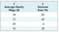
The following data— from a study of four American manufacturing companies— are available for a simple linear regression analysis attempting to link average hourly wage (x) to employee turnover rates (y).a. Show the data in a scatter diagram and use the least squares criterion to find the slope
Refer to Exercise 3 where we are trying to link mortgage interest rate (x) to home sales (y). The estimated regression equation there was ŷ = 90 – 4x. Can we reject the null hypothesis that the population slope, is 0 at the 1% significance level? Explain the implications of your answer.
Refer to Exercise 4, where we are trying to link average hourly wage (x) to employee turnover (y). The estimated regression equation there was ŷ =139.2 – 6.7x. Can we reject the null hypothesis that the population slope is 0 at the 10% significance level? Explain the implications of your answer.
Refer to Exercise 5, where we are trying to link the unemployment rate (x) to the consumer confidence index (y). The estimated regression equation there was ŷ =162 – 12x. Can we reject the hypothesis that the population slope, , is 0 at the 5% significance level? Explain the implications of
Refer to Exercise 8 (hedge fund returns and administrator compensation). The estimated regression equation turned out to be ŷ = 2.2 – .55x. Is the sample slope (b = .55) “statistically significant” at the 5% significance level? Explain the implications of your answer.
Refer to Exercise 9 where we are trying to link customer waiting time (x) to customer satisfaction (y). The estimated regression equation turned out to be ŷ =126 – 1.8x. Is the sample slope (b = 1.8) significantly different from 0 at the 5% significance level? Explain the implications of your
Refer to Exercise 10 where we are trying to link the number of customer choices (x) and the level of customer confidence (y). The estimated regression equation turned out to be ŷ = 66 6.8x. Is the sample slope (b = – 6.8) significantly different from 0 at the 5% significance level? Explain the
Refer to Exercise 44. With the sample evidence available, could we reject a 1.0 null hypothesis at the 5% significance level?
Refer to Exercise 45. With the sample evidence available, could we reject a β = – 5.0 null hypothesis at the 5% significance level?
Refer to Demonstration Exercise 11.1, where we are trying to link tolerance for risk (x) to % of financial assets invested in the stock market (y). The estimated regression equation turned out to be ŷ = 20 3.5x. Show the 95% confidence interval estimate of the average (or expected) % of assets
Refer to Exercise 1, where we are trying to link daily temperature (x) and coffee sales (y). The estimated regression equation turned out to be ŷ = 660 – 6.8x. Show the 90% confidence interval estimate of average coffee sales for all days with a high temperature of 68 degrees.
For a simple linear regression analysis attempting to relate consumer confidence (y) to the unemployment rate (x), the following data are available:Show the data in a scatter diagram and use the least squares criterion to find the slope (b) and the intercept (a) for the best fitting line. Sketch
Refer to Exercise 2, where we are attempting to link a company’s annual R & D Budget (x) to the number of patents granted to researchers at the company (y). The estimated regression equation turned out to be ŷ = 3.5 – 1.0x. Show the 95% confidence interval estimate of the expected number
Refer to Exercise 4, where we are trying to link average hourly wage (x) to employee turnover (y). The estimated regression equation turned out to be ŷ = 139.2 – 6.7x. Show the 95% confidence interval estimate of the expected turnover rate for the population of all companies with an average
Refer to Exercise 8 (hedge fund returns and administrator compensation). The estimated regression equation turned out to be ŷ = 2.2 + .55x. Show the 95% confidence interval estimate of the expected compensation for the population of all hedge fund administrators whose hedge funds have a 10%
Refer to Exercise 10 (too much information). The estimated regression equation turned out to be ŷ = 66 – 6.8x. Show the 95% confidence interval estimate of the average confidence score for a population of shoppers who are presented with six alternatives.
Refer to Demonstration Exercise 11.1, where we are trying to link tolerance for risk (x) to % of financial assets invested in the stock market (y). The estimated regression equation turned out to be ŷ = 20 + 3.5x. Show the 95% prediction interval for the % of assets invested in the stock market
Refer to Exercise 1, where we are trying to link daily temperature (x) and coffee sales (y). The estimated regression equation turned out to be ŷ = 660 – 6.8x. Show the 95% prediction interval for coffee sales tomorrow, when the high temperature will be 68 degrees.
Refer to Exercise 2, where we are attempting to link a company’s annual R & D Budget (x) to the number of patents granted to researchers at the company (y). The estimated regression equation turned out to be ŷ = 3.5 + 1.0x. Show the 90% prediction interval for the number of patents granted
Refer to Exercise 4, where we are trying to link average hourly wage (x) to employee turnover (y). The estimated regression equation turned out to be ŷ = 139.2 – 6.7x. Show the 95% prediction interval estimate of the turnover rate for a particular company with an average hourly wage of
Refer to Exercise 8 (hedge fund returns and administrator compensation). The estimated regression equation turned out to be ŷ = – 2.2 + .55x. Show the 95% prediction interval estimate of the compensation for a particular hedge fund administrators whose hedge fund has a 10% return.
Refer to Exercise 10 (too much information). The estimated regression equation turned out to be ŷ = 66 – 6.8x. Show the 95% prediction interval estimate of the confidence score for a particular shopper who is presented with six alternatives.
Buyers from online mega retailer Amazon.com use a star rating to rate products and sellers. You plan to use simple linear regression to link average star rating (x) to average daily sales (y) for Amazon sellers of consumer electronics who have at least 1000 ratings. The following data are
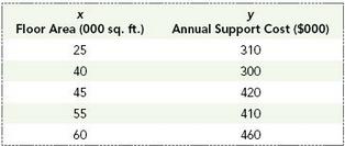
Plot the data and show the least squares line and the corresponding estimated regression equation. Given the line that you’ve drawn, about how much do support costs appear to increase with each 1000 square foot increase in floor area?Benton University is planning to construct a new sports complex
Compute the standard error of estimate (syx) for the least squares line you produced in Exercise 60. Benton University is planning to construct a new sports complex for use by its students. Beyond the cost of construction, support costs for things like staffing, heating, and general maintenance are
What proportion of the variation in annual support cost can be explained by the relationship between floor space and support cost that your line describes?Benton University is planning to construct a new sports complex for use by its students. Beyond the cost of construction, support costs for
Show that Total variation (SST) = Explained variation (SSR) + Unexplained variation (SSE).Benton University is planning to construct a new sports complex for use by its students. Beyond the cost of construction, support costs for things like staffing, heating, and general maintenance are of
Switching to the inference side of regression, a. Show the 95% confidence interval estimate of the population intercept.b. Show the 95% confidence interval estimate of the population slope. Explain what the interval means.c. Construct the appropriate hypothesis test to establish whether we can
Sticking to the inference side of regression, construct a 95% confidence interval estimate of E (y 50), the average building support cost for similar sports complexes having 50,000 square feet of floor area.
Benton’s sports complex will have 50,000 square feet of floor area. Show the 95% prediction interval for the support cost for Benton’s planned complex.
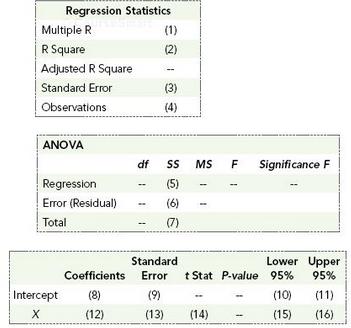
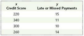
Using the Excel output template below, enter the correct values for each of the 16 missing values.Trenton Bank has a scoring system that it uses to evaluate new loan applications. You’ve been tracking the number of late or missed payments for a sample of “high risk” customers who received
Plot the data and show the least squares line and the corresponding estimated regression equation. Given the line you’ve drawn, about how much does the number of late or missed payments appear to fall as credit score increases by 100 points?Trenton Bank has a scoring system that it uses to
Compute the standard error of estimate (syx) for the least squares line you produced in Exercise 68. Trenton Bank has a scoring system that it uses to evaluate new loan applications. You’ve been tracking the number of late or missed payments for a sample of “high risk” customers who received
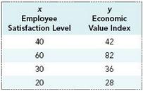
In a 2012 study, regression analysis was used to explore the possible connection between a firm’s overall employee satisfaction level and the firm’s market based economic value. Suppose the data for the study are given in the table below:Show the data in a scatter diagram and use the least
What proportion of the variation in the number of missed payments can be explained by the relationship between credit score and default rate that your line describes?Trenton Bank has a scoring system that it uses to evaluate new loan applications. You’ve been tracking the number of late or missed
Show that Total variation (SST) Explained variation (SSR) Unexplained variation (SSE).Trenton Bank has a scoring system that it uses to evaluate new loan applications. You’ve been tracking the number of late or missed payments for a sample of “high risk” customers who received loans and have
Switching to the inference side of regression, a. Show the 95% confidence interval estimate of the population intercept. b. Show the 95% confidence interval estimate of the population slope. c. Construct the appropriate hypothesis test to establish whether the coefficient for credit
Using the Excel output template shown in Exercise 67, enter the correct values for each of the 16 blanks indicated.Trenton Bank has a scoring system that it uses to evaluate new loan applications. You’ve been tracking the number of late or missed payments for a sample of “high risk” customers
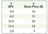
We would generally expect the share price of a company’s stock to be related to its reported earnings per share (EPS), the ratio of the company’s net income to the number of shares of stock outstanding. Below is a table showing the most recently reported EPS ratio and current share price for a
Suppose you have done a regression analysis on 50 data points in an attempt to find a linear connection between number of classes absent (x) and final exam score (y) for statistics students at State U. The correlation coefficient turned out to be .60. a. Discuss what the correlation coefficient
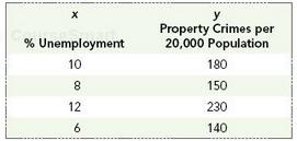
A recent article in a national business magazine reports that a strong linear connection appears to exist between regional unemployment rates and property crime. The following data were collected from four sample regions to support this position:The estimated regression equation turns out to be ŷ
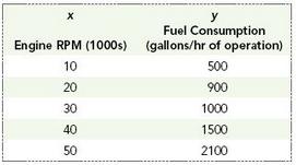
You are looking to use simple linear regression to link fuel consumption to revolutions per minute (RPM) for a new commercial jet aircraft engine that your company has produced. The following five observations are available from an early simulation:The estimated regression equation turns out to be
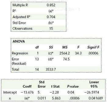
Partial regression results from a sample of 13 observations are shown below. Fill in the three missing values indicated by ()*. Is the coefficient for the variable x (9.16) statistically significant at the 1% significance level? Explain.
Partial regression results from a sample of 24 observations are shown below. Fill in the missing values indicated by ()*.
Hedge funds are sometimes referred to as “mutual funds for the super rich.” They are typically an aggressively managed portfolio of investments that require a very large initial investment. In a study using simple linear regression to examine how hedge fund performance is linked to the annual
Partial regression results from a sample of 15 observations are shown below. Fill in the missing values indicated by ()*. Can we use the sample results shown here to reject a β = 0 null hypothesis at the 5% significance level? Explain.
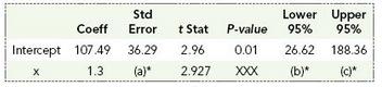
Partial regression results from a sample of 12 observations are shown below. Fill in the missing values indicated by ()*. Can we use the sample results shown here to reject a β = 0 null hypothesis at the 5% significance level? Explain
Partial regression results from a sample of 20 observations are shown below.a. Fill in the missing values indicated by ()*.Based on the printout, b. What % of the variation in the sample y values can be explained by the x to y relationship represented by the estimated regression line? c. Is the
For each of the following cases, report whether the coefficient for the variable x is significantly different from 0 at the 5% significance level and explain the implications of your decision.a. n = 13b. n = 19c. n = 25
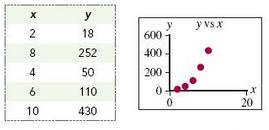
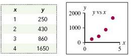
It is possible to adapt some of the tools used in linear regression to certain nonlinear cases. Suppose, for example, you wanted to link independent variable x to dependent variable y using the following data. The scatter diagram for the data is provided.The data here appear to suggest a nonlinear
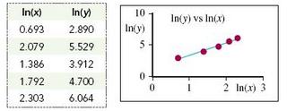
Suppose you suspect an exponential relationship between independent variable x and dependent variable y. (An exponential relationship has the general form y = mqx, where m and q are constants.) You want to use simple linear regression to estimate that relationship. You have the following data and
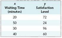
For most services, longer customer waiting times mean lower customer satisfaction. Suppose you have the following data to use for a simple linear regression analysis intended to link length of waiting time before speaking to a customer service representative (x) and customer satisfaction (y) for
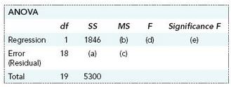
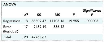
The following ANOVA table was produced in a simple linear regression analysis linking company profits (x) to shareholder dividends (y) for a sample of 2 β = 0companies. Notice that some of the entries in the table are missing.Fill in the missing values. Can we use the sample results represented
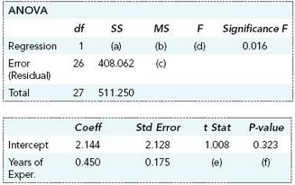
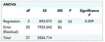
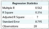
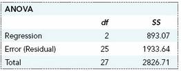
In a simple linear regression analysis attempting to link years of work experience (x) to salary (y), the following output was produced. Notice that some of the entries in the table are missing.Fill in the missing values and a. Use an F test to determine whether we can reject a β = 0 null
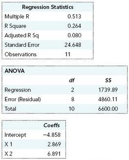
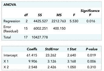
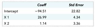
The output below is from a multiple linear regression analysis. The analysis attempts to link a dependent variable y to independent variables x1 and x2.a. Identify and interpret the estimated regression coefficients for x1 and x2.b. Identify and interpret the standard error of estimate. c.
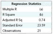
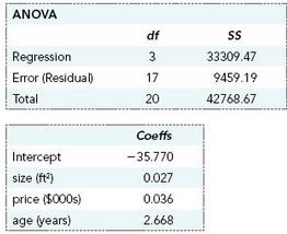
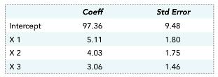
The output below is from a multiple linear regression analysis done by an area realty group. The analysis is intended to link y, the time that a house listed for sale remains on the market, to the size of the house (x1), the listing price (x2), and the age of the house (x3).a. Identify and
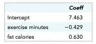
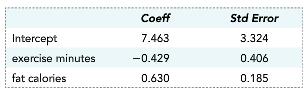
The output below is from a medical study that used multiple linear regression analysis to link monthly changes in weight (y = weight change in ounces) to daily exercise (x1 = minutes of strenuous daily exercise) and daily fat calorie intake (x2 = number of fat calories consumed
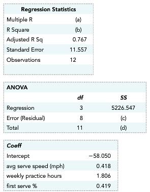
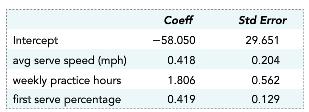
The output below is from a multiple linear regression analysis attempting to link winning percentage (y) to weekly practice time (x1), average speed of first serve (x2), and first serve percentage (x3) using data from a group of 12 professional tennis players over the past year.
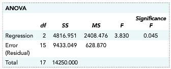
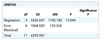
A regression analysis attempting to link dependent variable y to independent variables x1 and x2 produced the estimated regression equation ŷ = 59.89 + 8.11x1 + 5.67x2Below is the ANOVA table for the analysis.According to the ANOVA table, can we use sample results to reject an “all βs are
Below is the ANOVA table for the situation described in Exercise 13. It shows results from a regression analysis attempting to link y, the time that a house listed for sale remains on the market, to the size of the house (x1), the asking price (x2), and the age of the house (x3). Twenty-one
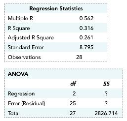
Below is the ANOVA table for the medical study described in Exercise 14. It shows results from a regression analysis attempting to link monthly weight change (y) to daily exercise minutes (x1) and daily fat calorie intake (x2) using a sample of 28 study participants. Notice that some
The output here is from the situation described in Exercise 15. There we were trying to link winning percentage (y) to daily practice time (x1), average speed of first serve (x2), and first serve percentage (x3) using data from a group of 12 professional tennis players over the past
Below are results from a regression analysis attempting to link a dependent variable y to independent variables x1 and x2.a. Can these results be used to reject the “all βs are 0” null hypothesis at the 5% significance level? Explain. b. Use t tests to determine which, if any, of the
Below is a table showing some of the results from the analysis described in Exercise 13, where we were attempting to link y, the time that a house listed for sale remains on the market, to the size of the house (x1), the asking price (x2), and the age of the house (x3). Twenty-one houses were
The following table shows some of the results from the multiple regression analysis described in Exercise 14 where we were attempting to link monthly changes in weight (y) to daily exercise time (x1) and daily intake of fat calories (x2), using a sample of 28 study participants.Use the appropriate
Below is a table showing some of the results from the multiple regression analysis described in Exercise 15. Here we were attempting to link winning percentage (y) to daily practice time (x1), average speed of first serve (x2), and first serve percentage (x3) based on data from a group of 12
Below is output from a regression analysis attempting to link dependent variable y to independent variables x1 and x2 using a sample of 19 observations. Build a 95% confidence interval estimate of the regression coefficients β1 and β2.
Below is output from a regression analysis attempting to link dependent variable y to three independent variables, x1, x2, and x3 based on a random sample of 20 observations. Build a 90% confidence interval estimate of the regression coefficients β1, β2 and β3.
The table shows some of the results from the multiple regression analysis described in Exercise 14. Here we were attempting to link monthly changes in weight (y) to daily exercise time (x1) and daily intake of fat calories (x2), using a sample of 28 study participants.Build a 95%
Below is a table showing some of the results from the multiple regression analysis described in Exercise 15. Here we were attempting to link winning percentage (y) to daily practice time (x1), average speed of first serve (x2), and first serve percentage (x3) using data from a group
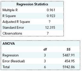
Below is output from a regression analysis attempting to link dependent variable y (productivity) to independent variables x1 (training time) and x2 (experience) using a sample of 20 assembly operators at Jensen Technologies. Compute the value of the adjusted r2.
Bigelow Roofing is developing a model to help its estimators bid on new roofing jobs. Below is output from a regression analysis attempting to link the dependent variable y (labor cost) to independent variables x1 (area of the roof), x2 (pitch of the roof), and x3 (number of special areas such as
The output below is from the regression analysis linking monthly changes in weight (y weight change in ounces) to daily exercise (x1 minutes of strenuous daily exercise) and daily fat calorie intake (x2 number of fat calories consumed daily). The sample consisted of 28 men in the 25 to 35 year age
The following output is from a study attempting to link monthly entertainment expenditures (y) for women aged 25 to 50 to two independent variables: age (x1) and monthly income (x2). Fill in the missing values.
Phillips Research plans to use a multiple regression model to connect a number of factors to the level of job satisfaction reported by individuals working in the computer science field. Phillips wants to include a categorical variable to indicate job level. This variable will classify job levels as

Showing 22500 - 22600 of 88243

First
219
220
221
222
223
224
225
226
227
228
229
230
231
232
233
Last

Step by Step Answers

Services

Sitemap
Fun
Definitions
Become Tutor
Used Textbooks
Study Help Categories
Recent Questions
Expert Questions
Campus Wear
Sell Your Books

Company Info

Security
Copyrights
Privacy Policy
Terms & Conditions
SolutionInn Fee
Scholarship
Online Quiz
Give Feedback, Get Rewards

Get In Touch

About Us
Contact Us
Career
Jobs
FAQ
Student Discount
Campus Ambassador

Secure Payment

Download Our App

© 2026 SolutionInn. All Rights Reserved