New Semester
Started
Get
50% OFF
Study Help!
--h --m --s
Claim Now
Question Answers
Textbooks
Find textbooks, questions and answers
Oops, something went wrong!
Change your search query and then try again
S
Books
FREE
Study Help
Expert Questions
Accounting
General Management
Mathematics
Finance
Organizational Behaviour
Law
Physics
Operating System
Management Leadership
Sociology
Programming
Marketing
Database
Computer Network
Economics
Textbooks Solutions
Accounting
Managerial Accounting
Management Leadership
Cost Accounting
Statistics
Business Law
Corporate Finance
Finance
Economics
Auditing
Tutors
Online Tutors
Find a Tutor
Hire a Tutor
Become a Tutor
AI Tutor
AI Study Planner
NEW
Sell Books
Search
Search
Sign In
Register
study help
Computer science
systems analysis and design
control system analysis and design
Control System Analysis And Design 2nd Edition A.K. Tripathi - Solutions
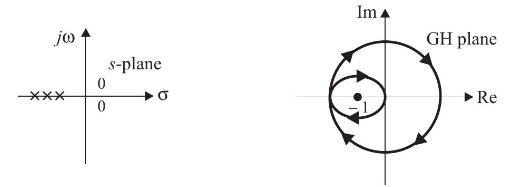
The pole-zero map and the Nyquist plot of the loop transfer function GH(s) of a feedback system are shown below. For this(a) both open loop and closed loop systems are stable.(b) open loop system is stable but closed loop system is unstable.(c) open loop system is unstable but closed loop system is
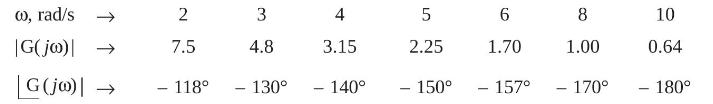
Consider the following open loop frequency response of a unity feedback system.The gain and phase margin of the system are respectively(a) \(0.00 \mathrm{~dB},-180^{\circ}\)(b) \(3.86 \mathrm{~dB},-180^{\circ}\)(c) \(0.00 \mathrm{~dB},-10^{\circ}\)(d) \(3.86 \mathrm{~dB}, 10^{\circ}\) w, rad/s
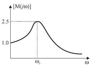
An underdamped second order system having a transfer function of the form \(\mathrm{M}(s)\) \(=\frac{K \omega_{n}^{2}}{s^{2}+2 \xi \omega_{n} s+\omega_{n}^{2}}\) has frequency response plot as shown below, then the system gain \(\mathrm{K}\) and the damping ratio approximately are(a)
The open loop transfer function of a unity feedback control system is given as \(\mathrm{G}(s)=\frac{a s+1}{s^{2}}\). The value of ' \(a\) ' to give a phase margin of \(45^{\circ}\) is equal to(a) 0.141(b) 0.441(c) 0.841(d) 1.141
A system has poles at \(0.01 \mathrm{~Hz}, 1 \mathrm{~Hz}\) and \(80 \mathrm{~Hz}\); zeros at \(5 \mathrm{~Hz}, 100 \mathrm{~Hz}\) and \(200 \mathrm{~Hz}\). The approximate phase of the system response at \(20 \mathrm{~Hz}\) is(a) \(-90^{\circ}\)(b) \(0^{\circ}\)(c) \(90^{\circ}\)(d)
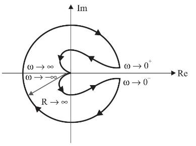
Consider the following Nyquist plot of a feedback system having open loop transfer function \(\mathrm{GH}(s)=(s+1) /\left[s^{2}(s-2)ight]\) as shown in the diagram given below. What is the number of closed loop poles in the right half of the \(s\) plane?(a) 0(b) 1(c) 2(d) 3 - (1) - -60-0 8 R Im (0)
Consider the following statements for a counter clockwise Nyquist path.1. For a stable closed loop system, the Nyquist plot of \(\mathrm{G}(s) \mathrm{H}(s)\) should encircle \((-1, j 0)\) point as many times as there are poles of \(\mathrm{G}(s) \mathrm{H}(s)\) in the right half of the \(s\)
The gain margin of a unity feedback control system with the open loop transfer function \(\mathrm{G}(s)=\frac{s+1}{s^{2}}\) is(a) 0(b) \(1 / \sqrt{2}\)(c) \(\sqrt{2}\)(d) \(\infty\)
In the \(\mathrm{GH}(s)\) plane, the Nyquist plot of the loop transfer function \(\mathrm{G}(s) \mathrm{H}(s)=\frac{\pi e^{-0.25 s}}{s}\) passes through the negative real axis at the point(a) \((-0.25, j 0)\)(b) \((-0.5, j 0)\)(c) \((-1, j 0)\)(d) \((-2, j 0)\)
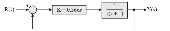
If the compensated system shown in figure has a phase margin of \(60^{\circ}\) at the crossover frequency of \(1 \mathrm{rad} / \mathrm{sec}\), the value of the gain \(\mathrm{K}\) is(a) 0.366(b) 0.732(c) 1.366(d) 2.738 R(S) + K + 0.366s 1 s(s+1) Y(s)
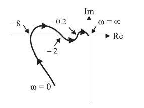
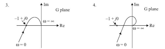
The polar diagram of a conditionally stable system for open loop gain \(K=1\) is shown in figure. The open loop transfer function of the system is known to be stable. The closed loop system is stable for(a) \(\mathrm{K}(b) \(\mathrm{K}(c) \(\mathrm{K}(d) \(\mathrm{K}>1 / 8\) and \(\mathrm{K} - 8
The radius of constant \(\mathrm{N}\) circle of \(\mathrm{N}=1\), is(a) 2(b) \(\sqrt{2}\)(c) 1(d) \(1 / \sqrt{2}\).
A constant \(\mathrm{M}\) circle is described by equation\[x^{2}+2.25 x+y^{2}=-11.25\]where \(x=\operatorname{Re}[\mathrm{G}(j \omega)]\) and \(y=\operatorname{Im}[\mathrm{G}(j \omega)]\). The value of \(\mathrm{M}\), is(a) 1(b) 2(c) 3(d) 4.
A constant \(\mathrm{N}\) circle has centre at \(-\frac{1}{2}+j 0\) in \(\mathrm{G}(j \omega)\) plane. It represents phase angle equal to(a) \(180^{\circ}\)(b) \(90^{\circ}\)(c) \(45^{\circ}\)(d) \(0^{\circ}\).
The \(\mathrm{N}\) loci is described by equation\[x^{2}+x+y^{2}=0 \text { where } x=\operatorname{Re}[\mathrm{G}(j \omega)] \text { and } y=\operatorname{Im}[\mathrm{G}(j \omega)] \text {. }\]The value of phase angle, is(a) \(-45^{\circ}\)(b) \(0^{\circ}\)(c) \(45^{\circ}\)(d) \(90^{\circ}\).
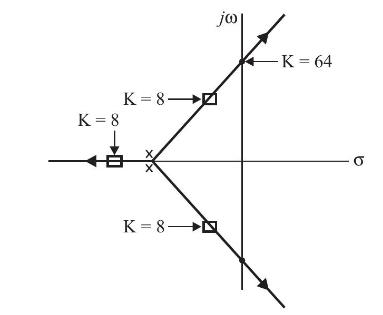
The root locus of a unity feedback system is shown in figure below. For design value of gain \(\mathrm{K}=8\), the root locations are shown by small square. The gain margin of system is(a) 2(b) 4(c) 6(d) 8. K = 8 K=8- K=8- jo| 3 - K = 64
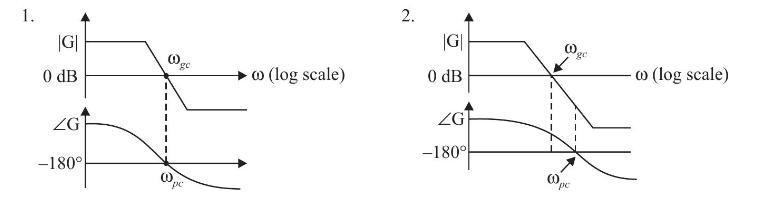
Consider the following plots.The plots which represent marginally stable systems, would include(a) 1 and 2(b) 3 and 4(c) 1 and 3(d) 2 and 4. 1. |G| 0 dB ZG -180 (0 ge pe co (log scale) 2. |G| 0 dB ZG -180 (0) pe ge w (log scale)
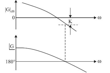
The Bode plots of an open loop transfer function of a control system are shown in figure below. The gain margin of the system is(a) \(\mathrm{K}\)(b) \(-\mathrm{K}\)(c) \(1 / \mathrm{K}\)(d) \(-1 / \mathrm{K}\) GdB 0 G 180 I I K (0) (0)
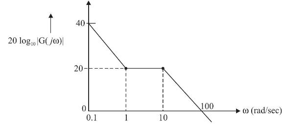
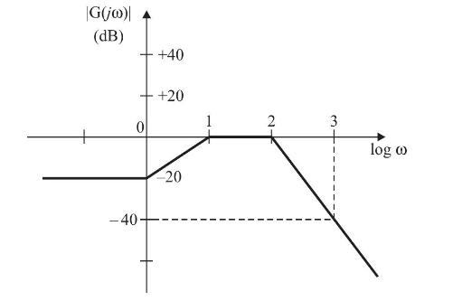
The \(\mathrm{dB}\) (Bode plot) of transfer function \(\mathrm{G}(\mathrm{s})\) is shown in figure below.Now, consider the following statements.I. \(\mathrm{G}(s)\) has corner frequencies at \(\omega=0.1,1\) and 10 .II. \(\mathrm{G}(s)=\frac{100(s+1)}{s(s+10)}\).III. The magnitude, \(20 \log
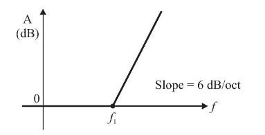
The function \(\mathrm{A}(f)\) corresponding to Bode plot of shown below is(a) \(\mathrm{A}(f)=j f / f\)(b) \(\mathrm{A}(f)=1 /\left(1-j f_{1} / fight)\)(c) \(\mathrm{A}(f)=1 /\left(1+j f / f_{1}ight)\)(d) \(\mathrm{A}(f)=1+j f / f_{1}\). A (dB) fi Slope = 6 dB/oct f
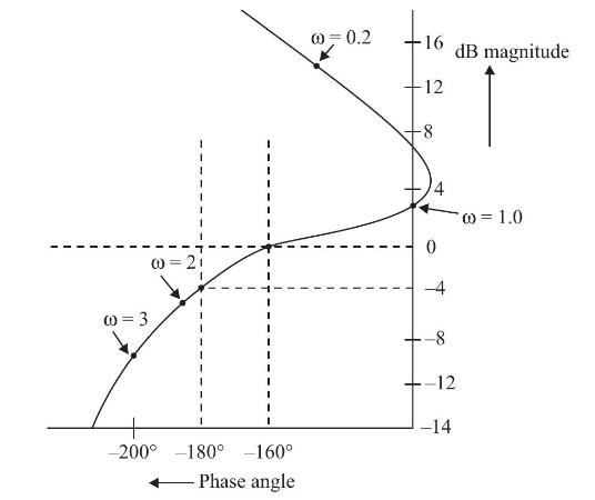
The \(\mathrm{dB}\) magnitude-phase angle plot for a typical open loop transfer function is shown below. Gain margin and phase margin respectively are(a) \(4 \mathrm{~dB}, 20^{\circ}\)(b) \(-4 \mathrm{~dB},-20^{\circ}\)(c) \(-4 \mathrm{~dB}, 20^{\circ}\)(d) \(4 \mathrm{~dB},-20^{\circ}\) (0=3 @= 21
The Bode \(\mathrm{dB}\) plot is shown below. The corresponding transfer function model is(a) \(\frac{10^{4}(1+j \omega)}{(10+j \omega)(100+j \omega)^{2}}\)(b) \(\frac{10^{-1}(1+j \omega)}{(10+j \omega)(100+j \omega)^{2}}\)(c) \(\frac{10^{-4}(1+j \omega)}{j \omega(j \omega+100)^{2}}\)(d)
If \(x=\operatorname{Re}[G(j \omega)]\) and \(y=\operatorname{Im}[\mathrm{G}(j \omega)]\), then for \(\omega ightarrow 0^{+}\), the Nyquist plot for \(\mathrm{G}(s)=1 / \mathrm{s}(s+1)(s+2)\), is(a) \(x=0\)(b) \(x=-3 / 4\)(c) \(x=y-(1 / 6)\)(d) \(x=y / \sqrt{3}\)
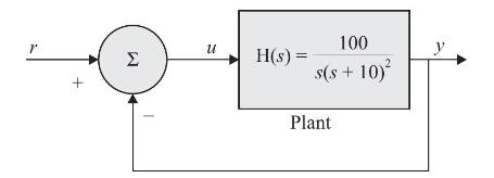
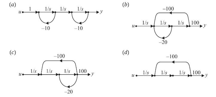
The input-output transfer function of a plant \(\mathrm{H}(s)=\frac{100}{s(s+10)^{2}}\). The plant is placed in a unity negative feedback configuration as shown in the figure below.The gain margin of the system under closed loop unity negative feedback is(a) \(0 \mathrm{~dB}\)(b) \(20
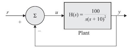
The input-output transfer function of a plant \(\mathrm{H}(s)=\frac{100}{s(s+10)^{2}}\). The plant is placed in a unity negative feedback configuration as shown in the figure below.The signal flow graph that DOES NOT model the plant transfer function \(\mathrm{H}(s)\) is T + U H(s) = 100 s(s + 10)
Construct simulation diagram in phase variable form for systems with following transfer functions and develop state space model in matrix form.(a) \(\mathrm{T}(s)=\frac{\mathrm{Y}(s)}{\mathrm{U}(s)}=\frac{11 s}{s^{3}+4 s^{2}+3 s+2}\)(b)
Construct simulation diagram in dual phase variable form for systems with following transfer functions and develop state space model in matrix form.(a) \(\mathrm{T}(\mathrm{s})=\frac{\mathrm{Y}(s)}{\mathrm{U}(s)}=\frac{2 s+6}{3 s^{3}+2 s^{2}+8 s+10}\)(b)
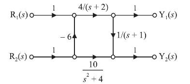
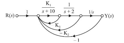
Develop state space model for the system with signal flow graph shown in Fig. P7.3. R(s) o R(s) o 1 - 64 4/(s + 2) 10 2+4 1 1/(s + 1) 1 -OY, (s) -0 Y(s)
Find diagonal state equations for a system with transfer function\[\mathrm{T}(s)=\frac{\mathrm{Y}(s)}{\mathrm{R}(s)}=\frac{s^{3}+18 s^{2}+50 s+50}{(s+3)(s+4)(s+5)}\]
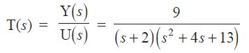
The SISO system with transfer functioninvolves complex characteristic roots. Obtain the diagonal form of state space model. Also obtain an alternative block diagonal model which does not involve complex numbers.Solution: Expand the transfer function in partial fractions to get Y(s) T(s) U(s) 9
The SISO system with repeated characteristic roots is described by transfer function\[\mathrm{T}(s)=\frac{\mathrm{Y}(s)}{\mathrm{U}(s)}=\frac{7 s^{3}}{(s+2)^{2}(s+6)^{2}}\]Find state space model in block diagonal Jordan canonical form.
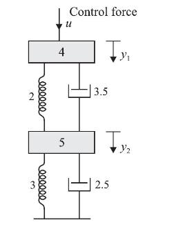
Construct state space model for the mechanical system shown in Fig. P7.7. N oooooo 000000 4 Control force U 5 3.5 Y Ty 2.5
Find characteristic equation for each of the following systems. Then for each, determine if they are stable.(a) \(\left[\begin{array}{l}\dot{x}_{1} \\ \dot{x}_{2} \\ \dot{x}_{3}\end{array}ight]=\left[\begin{array}{rrr}-2 & 0 & 1 \\ 0 & 0 & 1 \\ 0 & -10 &
The following transfer functions do not share a common denominator polynomial, but they may be made to do so by multiplying their numerators and denominators by appropriate factors. Obtain simulation diagram involving only three integrators. Then obtain state space model in matrix
Find decoupled state equations for the system described as\[\begin{aligned}{\left[\begin{array}{l}\dot{x}_{1} \\\dot{x}_{2}\end{array}ight] } & =\left[\begin{array}{rr}0 & 1 \\-6 & -5\end{array}ight]\left[\begin{array}{l}x_{1} \\x_{2}\end{array}ight]+\left[\begin{array}{ll}1 & 0 \\0 &
Obtain controllability and observability matrices and investigate whether or not the following systems are completely controllable and/or completely observable.(a) \(\left[\begin{array}{l}\dot{x}_{1} \\ \dot{x}_{2} \\ \dot{x}_{3}\end{array}ight]=\left[\begin{array}{rrr}1 & 0 & -2 \\ 3 &
Find the state response and system response for the systems described as follows:(a) \(\left[\begin{array}{l}\dot{x}_{1} \\ \dot{x}_{2}\end{array}ight]=\left[\begin{array}{ll}-4 & 1 \\ -3 & 0\end{array}ight]\left[\begin{array}{l}x_{1} \\ x_{2}\end{array}ight]+\left[\begin{array}{l}1 \\
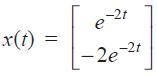
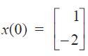
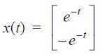
A system modelled as˙x(t)=Ax(t)x˙(t)=Ax(t)generates state response for initial vector Missing \end{array} and for Missing \end{array}. Find the system matrix A and state transition matrix (STM). x(t) = -21 -2e-21
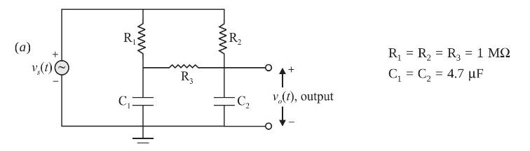
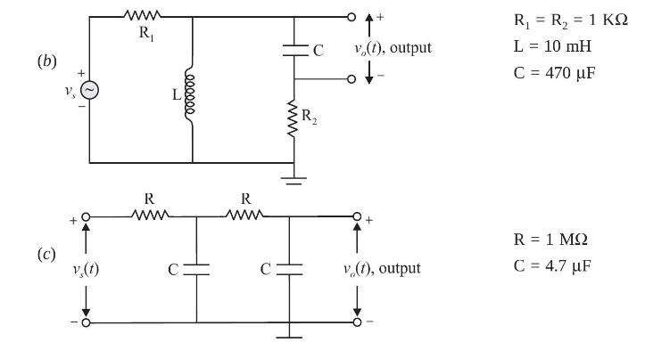
Develop state space model for each of the electrical networks shown below. Investigate if each one of them is completely controllable and/or completely observable. Substantiate the result with suitable comments if any. (a) v(1) www R C: m R www R C + v (t), output R = R = R = = 1 C C = 4.7 uF
A system using state feedback is governed by the following set of equations:\[\begin{aligned}{\left[\begin{array}{l}\dot{x}_{1} \\\dot{x}_{2} \\\dot{x}_{3}\end{array}ight] } & =\left[\begin{array}{rrr}0 & 1 & 0 \\0 & 0 & 1 \\-10 & -5 & -2\end{array}ight]\left[\begin{array}{l}x_{1} \\x_{2}
A system with state feedback is depicted below in Fig. P7.16. Find the values of \(K_{1}, K_{2}\) and \(\mathrm{K}_{3}\) so that the system satisfies the following performance requirements\[\begin{aligned}\text { Peak overshoot } & \leq 15 \% \\\text { Settling time } & \leq 4 \mathrm{sec}
For the system given below, an observer is to be designed to estimate the state variables. Select the observer gain and write the equations describing the observer dynamics. Also develop the block diagram for the interconnected system and observer.\[\left[\begin{array}{l}\dot{x}_{1}
Find diagonal state equations for a system with transfer function\[\mathrm{T}(s)=\frac{\mathrm{Y}(s)}{\mathrm{R}(s)}=\frac{2 s^{2}+3 s-7}{(s+2)\left(s^{2}+13 s+40ight)}\]
Construct phase variable form simulation diagram for the following transfer functions and develop state space model in matrix form(a) \(\mathrm{T}(s)=\frac{\mathrm{Y}(s)}{\mathrm{U}(s)}=\frac{10 \mathrm{~s}}{s^{3}+12 s^{2}+7 s+2}\)(b) Two outputs:\[\begin{aligned}&
Determine the transfer functions for the system modelled as[˙x1˙x2]=[01−3−7][x1x2]+[024−8][u1u2]y=[1−4][x1x2][˙x1˙x2]=[01−3−7][x1x2]+[024−8][u1u2]y=[1−4][x1x2]
Construct dual phase variable form simulation diagram for the following transfer functions and develop state space model in matrix form.(a) \(\frac{\mathrm{Y}(s)}{\mathrm{R}(s)}=\mathrm{T}(s)=\frac{2 s+8}{3 s^{3}+7 s^{2}+8 s+2}\)(b) Two inputs:\[\begin{aligned}&
Given a system\[\begin{aligned}{\left[\begin{array}{l}\dot{x}_{1} \\\dot{x}_{2} \\\dot{x}_{3}\end{array}ight] } & =\left[\begin{array}{rrr}0 & -2 & 3 \\0 & -4 & -1 \\0 & 1 & -8\end{array}ight]\left[\begin{array}{l}x_{1} \\x_{2} \\x_{3}\end{array}ight]+\left[\begin{array}{r}2 \\-8
Consider the following SISO system with complex characteristic roots. Develop state space model in matrix form with diagonal state equations. Also find block diagonal model involving real numbers.T(s)=Y(s)U(s)=2s2+3s−4(s+2)(s2+6s+10)T(s)=Y(s)U(s)=2s2+3s−4(s+2)(s2+6s+10)
Obtain controllability and observability matrices and investigate whether or not the following system is completely controllable and/or completely observable.\[\begin{aligned}& {\left[\begin{array}{l}\dot{x}_{1} \\\dot{x}_{2} \\\dot{x}_{3}\end{array}ight]=\left[\begin{array}{rrr}3 & 0 & -5 \\-2 & 1
The systems together with inputs and initial conditions are given below. Determine system response in each.(a) \(\quad \dot{x}=-2 x+3 r(t)\)\[y=4 x\]\[\begin{aligned}x(0) & =10 \\r(t) & =5 u(t)\end{aligned}\](b) \(\left[\begin{array}{l}\dot{x}_{1} \\
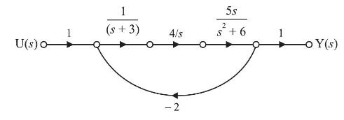
A system is described by the following signal flow graph. Write state and output equations in matrix form: U(s) c (s + 3) 4/s - 2 5s 2 S +6 -o Y(s)
A system using state feedback control is governed by the following set of equations. Determine feedback gains so as to place the closed loop system poles at \(s=-4\) and \(-4 \pm j 2\).\[\begin{aligned}{\left[\begin{array}{l}\dot{x}_{1} \\\dot{x}_{2} \\\dot{x}_{3}\end{array}ight] } &
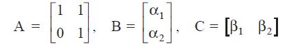
A system is described as follows:whereWhat restrictions should be imposed on α1,α2,β1α1,α2,β1 and β2β2 so that the system is completely controllable and observable. x y = Ax + Bu = Cx
The block diagram of a system together with state variable assignment as labelled therein, is shown in Fig. P7.12. Test controllability and observability. Comment on test result. U 3 1 s+2 1 S X +
For the system with matricesDesign an observer such that the observer eigen values are placed at ( −20,−20−20,−20 ). Develop observer equations and signal flow graph showing interconnection of system and observer. 0 1 0 A = B -10 -3 10 and C = [10]
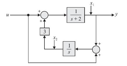
The state variable description of a single input single output linear system is given bywhereThe system is(a) Controllable and observable(b) Controllable but unobservable(c) Uncontrollable but observable(d) Uncontrollable and unobservable x(t) = Ax(t) + Bu(t) y(t) = Cx(t)
Which of the following properties are associated with the state transition matrix \(\phi(t)\) ?1. \(\phi\left(t_{1} / t_{2}ight)=\phi\left(t_{1}ight) \cdot \phi^{-1}\left(t_{2}ight)\)2. \(\phi(-t)=\phi^{-1}(t)\)3. \(\phi\left(t_{1}-t_{2}ight)=\phi\left(-t_{2}ight) \cdot \phi\left(t_{1}ight)\)Select
A linear system is described by the state equations\[\begin{aligned}{\left[\begin{array}{l}\dot{x}_{1} \\\dot{x}_{2}\end{array}ight] } & =\left[\begin{array}{ll}1 & 0 \\1 & 1\end{array}ight]\left[\begin{array}{l}x_{1} \\x_{2}\end{array}ight]+\left[\begin{array}{l}0 \\1\end{array}ight] r \\y &
Consider the following properties attributed to state model of a system.1. State model is unique.2. State model can be derived from the system transfer function.3. State model can be derived for time variant systems.Of these statements(a) 1, 2 and 3 are correct(b) 1 and 2 are correct(c) 2 and 3 are
A system is described by the state equation\[\left[\begin{array}{l}\dot{x}_{1} \\\dot{x}_{2}\end{array}ight]=\left[\begin{array}{ll}2 & 0 \\0 & 2\end{array}ight]\left[\begin{array}{l}x_{1} \\x_{2}\end{array}ight]+\left[\begin{array}{l}1 \\1\end{array}ight] u\]The state transition matrix of the
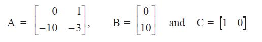
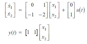
The state and output equations of a system areThe systems is(a) Neither state controllable nor output controllable(b) State controllable but not output controllable(c) Output controllable but not state controllable(d) Both state controllable and output controllable. x1 0 1 x1 + N-6-8-8 = y(t) =
The state equation of a linear system is given by \(\dot{x}=\mathrm{A} x+\mathrm{B} u\), where;\[A=\left[\begin{array}{rr}0 & 2 \\-2 & 0\end{array}ight] \text { and } B=\left[\begin{array}{r}0 \\-1\end{array}ight]\]The state transition matrix of the system is(a) \(\left[\begin{array}{cc}e^{2 t} & 0
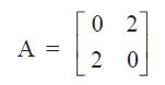
The state variable description of a linear autonomous system is ˙x=Axx˙=Ax where xx is a state vector andThe poles of the system are located at(a) -2 and +2(b) -2 and -2(c) −2j−2j and +2j+2j(d) +2 and +2 02 A = 2 0
Consider the Laplace transform of state transition matrix;\[\phi(s)=\left[\begin{array}{cc}\frac{s+6}{s^{2}+6 s+5} & \frac{1}{s^{2}+6 s+5} \\\frac{-5}{s^{2}+6 s+5} & \frac{s}{s^{2}+6 s+5}\end{array}ight]\]The eigen values of the system are(a) 0 and -6(b) 1 and -5(c) 0 and +6(d) -1 and -5
Which one of the following is NOT a correct statement about the state-space model of a physical system ?(a) State-space model can be obtained only for a linear system(b) Eigen values of the system represent the roots of the characteristic equation(c) \(\dot{x}=\mathrm{A} x+\mathrm{B} u\) represents
A linear second-order continuous time system is described by the following set of differential equations.\[\begin{aligned}\dot{x}_{1}(t) & =-2 x_{1}(t)+4 x_{2}(t) \\\dot{x}_{2}(t) & =-2 x_{1}(t)-x_{2}(t)+u(t)\end{aligned}\]where \(x_{1}(t)\) and \(x_{2}(t)\) are the state variables and \(u(t)\) is
For the system described by the state equation\[\dot{x}=\left[\begin{array}{ccc}0 & 1 & 0 \\0 & 0 & 1 \\0.5 & 1 & 2\end{array}ight] x+\left[\begin{array}{l}0 \\0 \\1\end{array}ight] u\]if the control signal \(u\) is given by \(u=\left[\begin{array}{lll}-0.5 & -3 & -5\end{array}ight] x+v\), then the
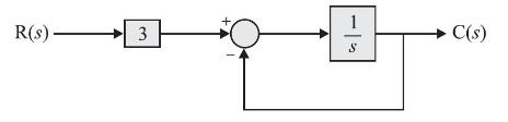
The matrix of any state-space equations for the transfer function \(C(s) / R(s)\) of the system, shown below in figure is(a) \(\left[\begin{array}{rr}-1 & 0 \\ 0 & -1\end{array}ight]\)(b) \(\left[\begin{array}{rr}0 & 1 \\ 0 & -1\end{array}ight]\)(c) \([-1]\)(d) [3] R(s)- 3 S C(s)
Given the homogeneous state-space equation \(\dot{x}=\left[\begin{array}{rr}-3 & 1 \\ 0 & -2\end{array}ight] x\). The steady state value of \(x_{s s}=\lim _{t ightarrow \infty} x(t)\), given the initial state value of \(x(0)=[10-10]^{t}\), \((t\) stands for transpose \()\) is(a)
The zero-input response of a system given by(a)(b)(c)(d) 1 0 N-HN = and 1 1 [x(0)] x2 (0) = 0 is:
The state-space representation in phase-variable form for the transfer function\[G(s)=\frac{2 s+1}{s^{2}+7 s+9} \quad \text { is }\](a) \(\dot{x}=\left[\begin{array}{rr}0 & 1 \\ -9 & -7\end{array}ight] x+\left[\begin{array}{l}0 \\ 1\end{array}ight] u: y=\left[\begin{array}{ll}1 & 2\end{array}ight]
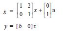
Letwhere bb is an unknown constant.This system is(a) observable for all values of bb(b) unobservable for all values of bb(c) observable for all non-zero values of bb(d) unobservable for all non-zero values of bb x+ 2 0 1 y= [b 0]x
Consider the following statements with respect to a system represented by its statespace model\[\dot{x}=\mathrm{A} x+\mathrm{B} u \text { and } y=\mathrm{C} x\]1. The state vector \(x\) of the system is unique.2. The eigen values of A are the poles of the system transfer function.3. The minimum
A state variable system \(\dot{x}(t)=\left[\begin{array}{rr}0 & 1 \\ 0 & -3\end{array}ight] x(t)+\left[\begin{array}{l}1 \\ 0\end{array}ight] u(t)\), with the initial condition \(x(0)=\left[\begin{array}{ll}-1 & 3\end{array}ight]^{\mathrm{T}}\) and the unit step input \(u(t)\) has.The state
A state variable system \(\dot{x}(t)=\left[\begin{array}{rr}0 & 1 \\ 0 & -3\end{array}ight] x(t)+\left[\begin{array}{l}1 \\ 0\end{array}ight] u(t)\), with the initial condition \(x(0)=\left[\begin{array}{ll}-1 & 3\end{array}ight]^{\mathrm{T}}\) and the unit step input \(u(t)\) has.The state
Consider the system \(s_{1}\) modelled as\[\dot{x}=\left[\begin{array}{rr}2 & 0 \\0 & -1\end{array}ight] x+\left[\begin{array}{l}1 \\0\end{array}ight] u\]and system \(s_{2}\) modelled as\[\dot{z}=\left[\begin{array}{ll}2 & 0 \\0 & 1\end{array}ight] z+\left[\begin{array}{l}1 \\0\end{array}ight]
Consider system \(s_{1}\) modelled as\[\begin{aligned}& \dot{x}=\left[\begin{array}{rr}2 & 0 \\0 & -1\end{array}ight] x+\left[\begin{array}{l}1 \\0\end{array}ight] u \\& y=\left[\begin{array}{ll}1 & 0\end{array}ight] x\end{aligned}\]and system \(s_{2}\) modelled as\[\begin{aligned}&
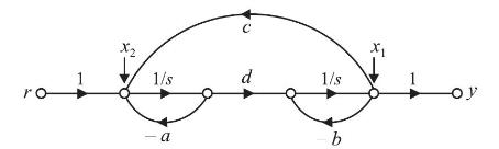
The signal flow graph together with state variable assignment is shown below:The condition for complete state controllability and complete observability is:(a) \(d eq 0\) and \(a, b, c\) can be anything.(b) \(a eq 0\) and \(b, c, d\) can be anything.(c) \(b eq 0\) and \(a, c, d\) can be
A system is described by state transition matrix \(\phi(t)=\left[\begin{array}{cc}e^{-t} & 0 \\ 0 & e^{-2 t}\end{array}ight]\) and has initial conditions \(\left[\begin{array}{l}x_{1}(0) \\ x_{2}(0)\end{array}ight]=\left[\begin{array}{l}1 \\ 2\end{array}ight]\). The state of system after 0.5
For the PD compensated system shown in Fig. P8.1, compute \(K\) and \(\mathbf{b}\) such that the system exhibits peak overshoot of \(2.5 \%\) and settling time of 0.5 seconds. R(s)- bs + + K s(s+12) Y(s)
A unity feedback system has open loop transfer function\[G(s)=\frac{K}{(s+3)(s+6)}\]and operates with peak overshoot of \(4.32 \%\). Design a PI compensator via root locus such that the system is forced to track the step input with zero error in steady state.
Design a lag-compensator for a unity feedback system with forward transmittance\[\mathrm{G}(s)=\frac{\mathrm{K}}{(s+1)(s+3)(s+5)}\]to yield the following specifications:(i) peak overshoot \(\leq 10 \%\)(ii) step error coefficient \(\geq 4\)
Design a cascade PD compensator for the unity feedback system with transmittance\[\mathrm{G}(s)=\frac{\mathrm{K}}{(s+2)^{2}(s+3)}\]so that the following design objectives are met:(i) \% peak overshoot \(=25 \%\)(ii) settling time, \(t_{s}=1.6\) seconds
For a system in unity feedback configuration with forward transmittance\[G(s)=\frac{K}{s^{2}},\]a cascade compensator is to be designed to achieve settling time of 1.6 seconds and peak overshoot of \(16 \%\). If the compensator zero is located at \(s=-1\), do the following:(a) Locate the dominant
Design PID compensator for the system with pole-zero function\[G(s)=\frac{K}{(s+3)(s+6)}\]in unity feedback configuration so as to meet the following specifications:Peak overshoot \(\leq 1.18 \%\)Settling time \(\leq 0.7\) secondsSteady state error for step input \(=0\)
A system in unity feedback configuration, has the transmittance\[G(s)=\frac{\mathrm{K}}{s(s+3)(s+9)}\](a) What value of \(\mathrm{K}\) will force the system to exhibit peak overshoot of \(20 \%\) to a step input?(b) For the value of \(\mathrm{K}\) found in (a), find the settling time, \(t_{s}\) and
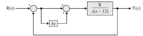
A system with transmittance\[\mathrm{G}(s)=\frac{\mathrm{K}}{s(s+6)^{2}}\]is placed in rate feedback control organisation as shown in Fig. P 8.8. Find \(\mathbf{K}\) and \(\mathbf{b}\) so as to meet the following design
A feedback compensated system is shown below. Do the following:(a) Find the value of \(\mathbf{a}\) and \(\mathbf{b}\) in minor feedback loop so as to achieve the settling time of 1 second with \(5 \%\) peak overshoot for the step response.(b) Find the value of \(\mathrm{K}\) so as to force the
Use frequency response methods to design a lag-compensator for a system in unity feedback configuration, with open loop transmittanceThe design goals are\[\mathrm{G}(s)=\frac{\mathrm{K}}{s(s+1)(0.2 s+1)}\](i) \(\mathrm{K}_{v}=10\)(ii) Phase margin \(\phi_{m s}=30^{\circ}\)
A unity feedback system has the loop transmittance\[\mathrm{G}(s)=\frac{1000 \mathrm{~K}}{s(s+40)(s+100)}\]Design a lead compensator so as to achieve the following specifications:(i) Peak overshoot \(=15 \%\)(ii) Error coefficient \(\mathrm{K}_{v}=40\)(iii) Peak time \(=0.1\) second.Use frequency
Use frequency response approach to design a lag-lead compensator for a unity feedback system where the loop transmittance is\[\mathrm{G}(s)=\frac{\mathrm{K}(s+8)}{s(s+4)(s+20)}\]The design goals are(i) peak overshoot \(=15 \%\)(ii) settling time \(=0.1 \mathrm{sec}\)(iii) velocity error coefficient
A system in unity feedback configuration, has the pole-zero function \(\frac{K}{s(s+50)(s+100)}\)Design the value of gain \(\mathrm{K}\) for \(15 \%\) peak overshoot in closed loop step response using frequency response techniques.
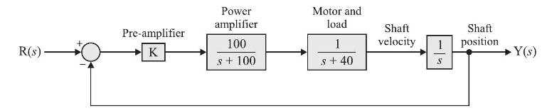
Design a PI compensator for the position control system shown in Fig. P 8.15, to achieve the following design goals:(i) Steady state error for ramp input =0=0(ii) Peak overshoot for step input =9.48%=9.48%Use frequency response approach. R(s) Pre-amplifier K Power amplifier 100 s + 100 Motor and
A unity feedback system with loop transmittance\[\mathrm{G}(s)=\frac{\mathrm{K}}{s(s+5)(s+20)}\]operates with approximately \(55 \%\) peak overshoot and 0.5 seconds peak time when the gain \(\mathrm{K}\) is adjusted to yield the velocity error coefficient \(\mathrm{K}_{v}=10\).Use frequency
A system in unity feedback configuration, has the transmittance\[\mathrm{G}(s)=\frac{\mathrm{K}}{(s+3)(s+9)(s+15)}\]Use frequency response methods to determine the value of K. Such that system is forced to exhibit(a) Gain margin of \(10 \mathrm{~dB}\).(b) Percent overshoot in step response of
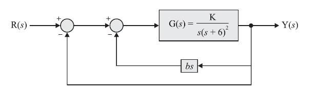
A system is placed in a feedback organisation as shown in Fig. D8.2. Design a lead compensator so as to meet the following design goals:(i) Error coefficient \(\mathrm{K}_{v}=2\)(ii) Phase margin \(\phi_{m}=30^{\circ}\) R(s) G(s) = K s(s+ 2) (s+4) (s + 6) Y(s)
The open loop transfer function of a system in unity feedback configuration, is\[\mathrm{G}(s)=\frac{\mathrm{K}}{(s+1)(s+2)(s+10)}\]Use the root locus approach to do the following:(a) Determine the value of \(\mathrm{K}\) such that system exhibits peak overshoot of \(57.2 \%\).(b) Find the steady
Use the root locus approach to design a lag compensator for the system of drill problem D8.3 to achieve the following design goals:(i) Peak overshoot ≤57.5%≤57.5%(ii) The steady state error for a step input =0.019=0.019
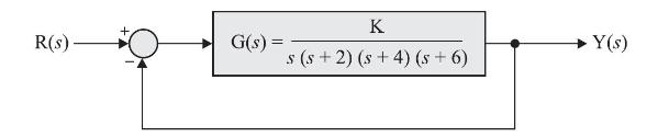
A system in unity feedback configuration, has the loop transmittance\[\mathrm{G}(s)=\frac{\mathrm{K}}{s(s+4)(s+6)}\]Use the root locus methods and do the following:(a) Sketch root locus and find the value of gain \(\mathrm{K}\) such that damping ratio, \(\xi=0.5\).(b) What is settling time of the
Design a lead compensator while using root locus for the system of drill problem D8.5, to meet the design specifications as follows:(i) Peak overshoot \(\leq 30 \%\)(ii) Settling time \(t_{\mathrm{s}} \leq 2\) seconds.
Showing 200 - 300
of 480
1
2
3
4
5
Step by Step Answers