New Semester
Started
Get
50% OFF
Study Help!
--h --m --s
Claim Now
Question Answers
Textbooks
Find textbooks, questions and answers
Oops, something went wrong!
Change your search query and then try again
S
Books
FREE
Study Help
Expert Questions
Accounting
General Management
Mathematics
Finance
Organizational Behaviour
Law
Physics
Operating System
Management Leadership
Sociology
Programming
Marketing
Database
Computer Network
Economics
Textbooks Solutions
Accounting
Managerial Accounting
Management Leadership
Cost Accounting
Statistics
Business Law
Corporate Finance
Finance
Economics
Auditing
Tutors
Online Tutors
Find a Tutor
Hire a Tutor
Become a Tutor
AI Tutor
AI Study Planner
NEW
Sell Books
Search
Search
Sign In
Register
study help
mathematics
first course differential equations
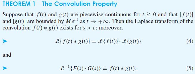
Differential Equations And Linear Algebra 4th Edition C. Edwards, David Penney, David Calvis - Solutions
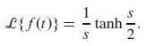
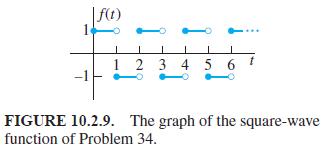
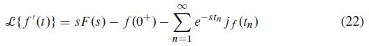
Apply the extension of Theorem 1 in Eq. (22) to derive the Laplace transforms given in Problems 32 through 37.If f(t) = (-1)[[t]] is the square-wave function whose graph is shown in Fig. 10.2.9, then L{f(t)} = - tanh S 2
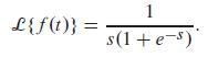
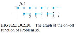
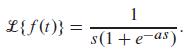
Apply the extension of Theorem 1 in Eq. (22) to derive the Laplace transforms given in Problems 32 through 37.If f (t) is the unit on–off function whose graph is shown in Fig. 10.2.10, then L{f(t)} 1 s(1 + e-s)
Use Laplace transforms to solve the initial value problems in Problems 27 through 38.x(4) + 13x" + 36x = 0; x (0) = x" (0) = 0, x' (0) = 2, x (3) (0) = -13
In Problems 31 through 35, the values of mass m, spring constant k, dashpot resistance c, and force f (t) are given for a mass–spring–dashpot system with external forcing function. Solve the initial value problemand construct the graph of the position function x(t). mx" + cx' + kx = f(t); x(0)
Derive the transform of f (t) = sinh k t by the method used in the text to derive the formula in (14).
In Problems 29 through 34, transform the given differential equation to find a nontrivial solution such that x(0) = 0.tx" + (4t - 2)x' + (13t - 4)x = 0
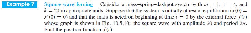
In Problems 36 and 37, a mass–spring–dashpot system with external force f (t) is described. Under the assumption that x(0) = x'(0) = 0, use the method of Example 7 to find the transient and steady periodic motions of the mass. Then construct the graph of the position function x(t). If you would
In Problems 31 through 35, the values of mass m, spring constant k, dashpot resistance c, and force f (t) are given for a mass–spring–dashpot system with external forcing function. Solve the initial value problemand construct the graph of the position function x(t). mx" + cx' + kx = f(t); x(0)
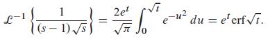
Apply the convolution theorem to show that 2et L 2-¹ { (s - D √✓s} = 2²/4 + √²/² S e-¹² du = e¹erf√i. π
Use Laplace transforms to solve the initial value problems in Problems 27 through 38.x(4) + 8x" + 16x = 0; x (0) = x' (0) = x" (0) = 0, x(3) (0) = 1
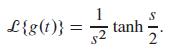
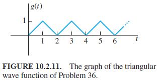
Apply the extension of Theorem 1 in Eq. (22) to derive the Laplace transforms given in Problems 32 through 37.If g(t) is the triangular wave function whose graph is shown in Fig. 10.2.11, then 1 L{g(t)} = tanh S
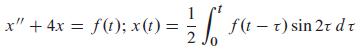
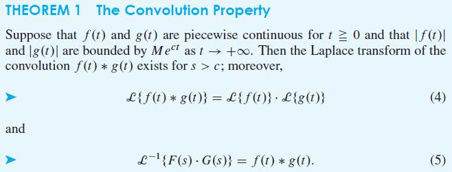
In Problems 36 through 38, apply the convolution theorem to derive the indicated solution x(t) of the given differential equation with initial conditions x(0) = x'(0) = 0. x" + 4x = f(t); x (t) = >= ²/6² f(t - t) sin 2t dt 2
Show that the function f(t) = sin(et2) is of exponential order as t → + ∞ but that its derivative is not.
In Problems 36 through 38, apply the convolution theorem to derive the indicated solution x(t) of the given differential equation with initial conditions x(0) = x'(0) = 0. x" + 2x + x = f(t); x(t) = 0 te tf(t-t) dt
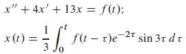
Use Laplace transforms to solve the initial value problems in Problems 27 through 38.x" + 4x' + 13x = te-t ; x(0) = 0, x' (0) = 2
In Problems 36 and 37, a mass–spring–dashpot system with external force f (t) is described. Under the assumption that x(0) = x'(0) = 0, use the method of Example 7 to find the transient and steady periodic motions of the mass. Then construct the graph of the position function x(t). If you would
In Problems 36 through 38, apply the convolution theorem to derive the indicated solution x(t) of the given differential equation with initial conditions x(0) = x'(0) = 0. x" + 4x + 13x = f(t); T x (t) = = f(1 - 7)e-2r sin 3x dr ² 1 3 J
Use Laplace transforms to solve the initial value problems in Problems 27 through 38.x" + 6x' + 18x = cos 2t ; x (0) = 1, x'(0) = -1
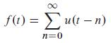
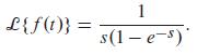
The unit staircase function is defined as follows:(a) Sketch the graph of f to see why its name is appropriate.(b) Show thatfor all t ≧ 0.(c) Assume that the Laplace transform of the infinite series in part (b) can be taken termwise (it can). Apply the geometric series to obtain the result f(t) =
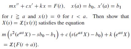
Suppose the function x(t) satisfies the initial value problem mx" + cx' + kx = F(t), x(a) = bo, x'(a) = b₁ for ta and x(t) = 0 for t < a. Then show that X(s) = L{x (t)} satisfies the equation m (5² (eas X) - sbo-b₁) + c(s(eas X) - bo) + k (eas X) = L{F(t + a)}.
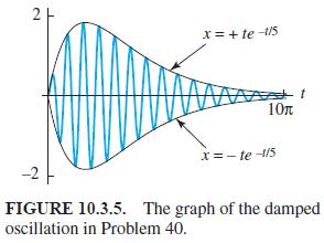
Problems 39 and 40 illustrate two types of resonance in a mass–spring–dashpot system with given external force F(t) and with the initial conditions x(0) = x'(0) = 0.Suppose that m = 1, k = 9.04, c = 0.4, and F(t) = 6e-t/5 cos 3t. Derive the solutionShow that the maximum value of the amplitude
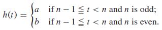
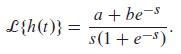
Given constants a and b, define h(t) for t ≧ 0 bySketch the graph of h and apply one of the preceding problems to show that h(t) = if n-1 ≤ t
Differentiate termwise the series for J0(x) to show directly that J'0(x) = -J1(x) (another analogy with the cosine and sine functions).
If x = a ≠ 0 is a singular point of a second-order linear differential equation, then the substitution t = x - a transforms it into a differential equation having t = 0 as a singular point. We then attribute to the original equation at x = a the behavior of the new equation at t = 0. Classify (as
In Problems 1 through 8, determine whether x = 0 is an ordinary point, a regular singular point, or an irregular singular point. If it is a regular singular point, find the exponents of the differential equation at x = 0.x2 (1 - x2) y" + 2xy' - 2y = 0
Derive the recursion formula in Eq. (2) for Bessel’s equation. [(m + r)2 - p2]cm + Cm-2 = 0 (2)
Any integral of the form ∫ xm Jn (x) dx can be evaluated in terms of Bessel functions and the indefinite integral ∫ J0 (x) dx. The latter integral cannot be simplified further, but the function ∫x0 J0 (t) dt is tabulated in Table 11.1 of Abramowitz and Stegun. Use the identities in Eqs. (22)
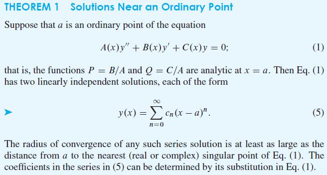
Find general solutions in powers of x of the differential equations in Problems 1 through 15. State the recurrence relation and the guaranteed radius of convergence in each case.y'' + xy = 0 (an Airy equation)
Any integral of the form ∫ xm Jn (x) dx can be evaluated in terms of Bessel functions and the indefinite integral ∫ J0 (x) dx. The latter integral cannot be simplified further, but the function ∫x0 J0 (t) dt is tabulated in Table 11.1 of Abramowitz and Stegun. Use the identities in Eqs. (22)
If x = a ≠ 0 is a singular point of a second-order linear differential equation, then the substitution t = x - a transforms it into a differential equation having t = 0 as a singular point. We then attribute to the original equation at x = a the behavior of the new equation at t = 0. Classify (as
Show (as in Example 3) that the power series method fails to yield a power series solution of the form y = Σ cnxn for the differential equations in Problems 15 through 18.xy' + y = 0 Example 3 Solve the equation x²y' = y - x - 1.
If x = a ≠ 0 is a singular point of a second-order linear differential equation, then the substitution t = x - a transforms it into a differential equation having t = 0 as a singular point. We then attribute to the original equation at x = a the behavior of the new equation at t = 0. Classify (as
If x = a ≠ 0 is a singular point of a second-order linear differential equation, then the substitution t = x - a transforms it into a differential equation having t = 0 as a singular point. We then attribute to the original equation at x = a the behavior of the new equation at t = 0. Classify (as
Show (as in Example 3) that the power series method fails to yield a power series solution of the form y = Σ cnxn for the differential equations in Problems 15 through 18.2xy' = y Example 3 Solve the equation x²y' = y - x - 1.
Any integral of the form ∫ xm Jn (x) dx can be evaluated in terms of Bessel functions and the indefinite integral ∫ J0 (x) dx. The latter integral cannot be simplified further, but the function ∫x0 J0 (t) dt is tabulated in Table 11.1 of Abramowitz and Stegun. Use the identities in Eqs. (22)
Use power series to solve the initial value problems in Problems 16 and 17.(1 + x2) y" + 2xy' - 2y = 0; y(0) = 0, y'(0) = 1
Show (as in Example 3) that the power series method fails to yield a power series solution of the form y = Σ cnxn for the differential equations in Problems 15 through 18.x2y' + y = 0 Example 3 Solve the equation x²y' = y - x - 1.
Any integral of the form ∫ xm Jn (x) dx can be evaluated in terms of Bessel functions and the indefinite integral ∫ J0 (x) dx. The latter integral cannot be simplified further, but the function ∫x0 J0 (t) dt is tabulated in Table 11.1 of Abramowitz and Stegun. Use the identities in Eqs. (22)
Find two linearly independent Frobenius series solutions (for x > 0) of each of the differential equations in Problems 17 through 26.4xy'' + 2y' + y = 0
Solve the initial value problems in Problems 18 through 22. First make a substitution of the form t = x - a, then find a solution Σcntn of the transformed differential equation. State the interval of values of x for which Theorem 1 of this section guarantees convergence.y" + (x - 1) y' + y = 0;
Show (as in Example 3) that the power series method fails to yield a power series solution of the form y = Σ cnxn for the differential equations in Problems 15 through 18.x3y' = 2y Example 3 Solve the equation x²y' = y - x - 1.
Find two linearly independent Frobenius series solutions (for x > 0) of each of the differential equations in Problems 17 through 26.2xy'' + 3y' - y = 0
In Problems 19 through 30, express the general solution of the given differential equation in terms of Bessel functions.x2y'' - xy' + (1 + x2)y = 0
Solve the initial value problems in Problems 18 through 22. First make a substitution of the form t = x - a, then find a solution Σcntn of the transformed differential equation. State the interval of values of x for which Theorem 1 of this section guarantees convergence.(2x - x2) y" - 6(x - 1) y'
In Problems 19 through 22, first derive a recurrence relation giving cn for n ≧ 2 in terms of c0 or c1 (or both). Then apply the given initial conditions to find the values of c0 and c1. Next determine cn (in terms of n, as in the text) and, finally, identify the particular solution in terms of
Find two linearly independent Frobenius series solutions (for x > 0) of each of the differential equations in Problems 17 through 26.2xy'' - y' - y = 0
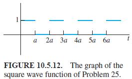
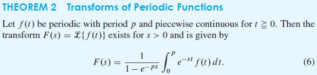
Apply Theorem 2 to show that the Laplace transform of the square wave function of Fig. 10.5.12 is L{f(t)} = 1 s(1+e-as)'
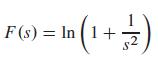
Find the inverse transforms of the functions in Problems 23 through 28. F(s) = In s² +1 (s + 2)(s-3)
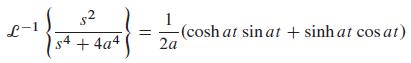
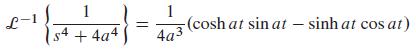
Use the factorizationto derive the inverse Laplace transforms listed in Problems 23 through 26. s4 + 4a4 = (s² - 2as +2a²) (s² + 2as + 2a²) ($2
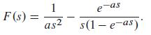
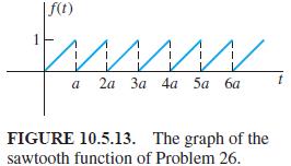
Apply Theorem 2 to show that the Laplace transform of the sawtooth function f (t) of Fig. 10.5.13 is F(s) = 1 as2 e as s(1-e-as)*
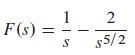
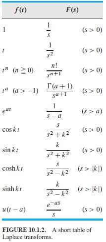
Use the transforms in Fig. 10.1.2 to find the inverse Laplace transforms of the functions in Problems 23 through 32. F(s) = 1 S 2 85/2
Find the inverse transforms of the functions in Problems 23 through 28. F(s) = tan 1 3 s+2
Use the factorizationto derive the inverse Laplace transforms listed in Problems 23 through 26. s4 + 4a4 = (s² - 2as +2a²) (s² + 2as + 2a²) ($2
Use the transforms in Fig. 10.1.2 to find the inverse Laplace transforms of the functions in Problems 23 through 32. F(s) = 1 S+5
Find the inverse transforms of the functions in Problems 23 through 28. F (s) = ln (1 + -3/2)
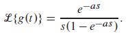
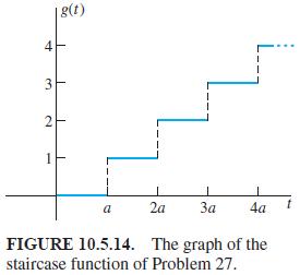
Let g(t) be the staircase function of Fig. 10.5.14. Show that g(t) = (t/a) - f(t), where f is the sawtooth function of Fig. 10.5.14, and hence deduce that L{g(t)} e -as s(1-e-as)
Use Laplace transforms to solve the initial value problems in Problems 27 through 38.x" + 6x' + 25x = 0; x (0) = 2, x' (0) = 3
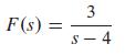
Use the transforms in Fig. 10.1.2 to find the inverse Laplace transforms of the functions in Problems 23 through 32. F(s) = 3 S-4
Find the inverse transforms of the functions in Problems 23 through 28. F(s) = S (s² + 1)3 2
Apply Theorem 1 as in Example 5 to derive the Laplace transforms in Problems 28 through 30. L{t cos kt} = s²-k² (s²+k²)²
Suppose that f(t) is a periodic function of period 2a with f(t) = t if 0 ≦ t < a and f (t) = 0 if a ≦ t < 2a. Find ℒ {f (t)}.
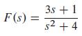
Use the transforms in Fig. 10.1.2 to find the inverse Laplace transforms of the functions in Problems 23 through 32. F(s) = 3s +1 s² +4
Use Laplace transforms to solve the initial value problems in Problems 27 through 38.x" - 6x' + 8x = 2; x (0) = x'(0) = 0
In Problems 29 through 34, transform the given differential equation to find a nontrivial solution such that x(0) = 0.tx'' + (t - 2)x' + x = 0
Apply Theorem 1 as in Example 5 to derive the Laplace transformsin Problems 28 through 30. £{t sinhkt}= 2ks (s²-k²)2
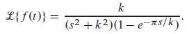
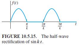
Suppose that f (t) is the half-wave rectification of sin kt , shown in Fig. 10.5.15. Show that L{f(t)} = k (s2+k²)(1-e-ns/k)*
Use Laplace transforms to solve the initial value problems in Problems 27 through 38.x" - 4x = 3t; x (0) = x'(0) = 0
Use the transforms in Fig. 10.1.2 to find the inverse Laplace transforms of the functions in Problems 23 through 32. F(s) = 5-3s s² +9
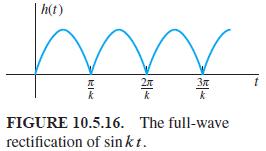
Let g(t) = u(t - π/k) f (t - π/k), where f(t) is the function of Problem 29 and k > 0. Note that h(t) = f(t) + g(t) is the full-wave rectification of sin kt shown in Fig. 10.5.16. Hence deduce from Problem 29 that.Problem 29Suppose that f (t) is the half-wave rectification of sin kt , shown in
In Problems 29 through 34, transform the given differential equation to find a nontrivial solution such that x(0) = 0.tx'' + (3t - 1)x' + 3x = 0
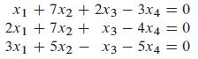
In Problems 19–22, reduce the given system to echelon form to find a single solution vector u such that the solution space is the set of all scalar multiples of u. 3x4 = 0 4x4 = 0 - 3x15x2x3 - 5x4 = 0 x1 + 7x2 + 2x3 2x17x2 + x3
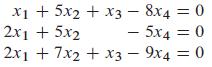
In Problems 19–22, reduce the given system to echelon form to find a single solution vector u such that the solution space is the set of all scalar multiples of u. x1 + 5x2 + x3 - 8x4 = 0 2x1 + 5x2 - 5x4 = 0 2x17x2 + x39x4 = 0
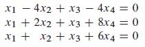
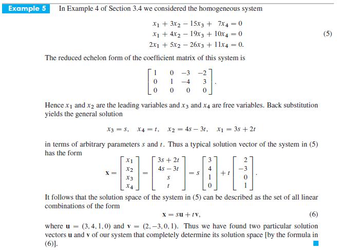
In Problems 15–18, apply the method of Example 5 to find two solution vectors u and v such that the solution space is the set of all linear combinations of the form su + tv. x14x2 + x3 4x4 = 0 x1 + 2x2 + x3 + 8x4 = 0 x₁ + x₂ + x3 + 6x4: 0
In Problems 1–14, a subset W of some n-space Rn is defined by means of a given condition imposed on the typical vector (x1 , x2 , .... ,xn). Apply Theorem 1 to determine whether or not W is a subspace of Rn.W is the set of all those vectors in R4 whose components are all nonzero.
In Problems 1–14, a subset W of some n-space Rn is defined by means of a given condition imposed on the typical vector (x1 , x2 , .... ,xn). Apply Theorem 1 to determine whether or not W is a subspace of Rn.W is the set of all vectors in R4 such that x1 x2 x3 x4 = 0.
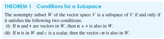
In Problems 1–14, a subset W of some n-space Rn is defined by means of a given condition imposed on the typical vector (x1 , x2 , .... ,xn). Apply Theorem 1 to determine whether or not W is a subspace of Rn.W is the set of all vectors in R4 such that x1 x2 = x3 x4. THEOREM 1
In Problems 1–14, a subset W of some n-space Rn is defined by means of a given condition imposed on the typical vector (x1 , x2 , .... ,xn). Apply Theorem 1 to determine whether or not W is a subspace of Rn.W is the set of all vectors in R4 such that x1 + x2 = x3 + x4. THEOREM 1
In Problems 1–14, a subset W of some n-space Rn is defined by means of a given condition imposed on the typical vector (x1 , x2 , .... ,xn). Apply Theorem 1 to determine whether or not W is a subspace of Rn.W is the set of all vectors in R2 such that |x1| + |x2| = 1. THEOREM 1
In Problems 1–14, a subset W of some n-space Rn is defined by means of a given condition imposed on the typical vector (x1 , x2 , .... , xn). Apply Theorem 1 to determine whether or not W is a subspace of Rn.W is the set of all vectors in R2 such that (x1)2 + (x2)2 = 1. THEOREM 1
In Problems 1–14, a subset W of some n-space Rn is defined by means of a given condition imposed on the typical vector (x1 , x2 , .... ,xn). Apply Theorem 1 to determine whether or not W is a subspace of Rn.W is the set of all vectors in R2 such that (x1)2 + (x2)2 = 0. THEOREM 1
In Problems 1–14, a subset W of some n-space Rn is defined by means of a given condition imposed on the typical vector (x1, x2, ....,xn). Apply Theorem 1 to determine whether or not W is a subspace of Rn.W is the set of all vectors in R2 such that |x1| = |x2|. THEOREM 1 Conditions for a
In Problems 1–14, a subset W of some n-space Rn is defined by means of a given condition imposed on the typical vector (x1 , x2 , .... ,xn). Apply Theorem 1 to determine whether or not W is a subspace of Rn.W is the set of all vectors in R4 such that x1 = 3x3 and x2 = 4x4. THEOREM 1
In Problems 1–14, a subset W of some n-space Rn is defined by means of a given condition imposed on the typical vector (x1, x2, ....,xn). Apply Theorem 1 to determine whether or not W is a subspace of Rn.W is the set of all vectors in R4 such that x1 + 2x2 + 3x3 + 4x4 = 0. THEOREM 1 Conditions
In Problems 1–14, a subset W of some n-space Rn is defined by means of a given condition imposed on the typical vector (x1 , x2 , .... ,xn). Apply Theorem 1 to determine whether or not W is a subspace of Rn.W is the set of all vectors in R3 such that x1 + x2 + x3 = 1. THEOREM 1
In Problems 1–14, a subset W of some n-space Rn is defined by means of a given condition imposed on the typical vector (x1 , x2 , .... ,xn). Apply Theorem 1 to determine whether or not W is a subspace of Rn.W is the set of all vectors in R3 such that x2 = 1. THEOREM 1 Conditions for a
In Problems 1–14, a subset W of some n-space Rn is defined by means of a given condition imposed on the typical vector (x1 , x2 , ....,xn). Apply Theorem 1 to determine whether or not W is a subspace of Rn.W is the set of all vectors in R3 such that x1 = 5x2. THEOREM 1 Conditions for a
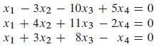
In Problems 15–26, find a basis for the solution space of the given homogeneous linear system. x13x2 x1 +4x2+ 11x3 x1 + 3x2 + 8x3 10x3 + 5x4 = 0 2x4 = 0 x4 = 0
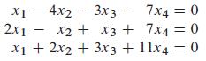
In Problems 15–26, find a basis for the solution space of the given homogeneous linear system. x14x2 3x3 - - + x3 + 7x4 = 0 2x1x₂ 7x4 = 0 X1 + 2x2 + 3x3 + 11x4 = 0 =
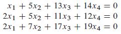
In Problems 15–26, find a basis for the solution space of the given homogeneous linear system. x1 + 5x2 + 13x3 + 14x4 = 0 2x1 + 5x2 + 11x3 + 12x4 = = 0 2x17x2 + 17x3 + 19x4 = 0
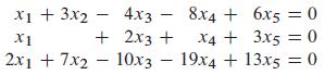
In Problems 15–26, find a basis for the solution space of the given homogeneous linear system. x1 + 3x2 - 4x3 X1 + 2x3 + 2x17x210x3 8x4 + 6x5 = 0 X4+ 3x50 19x4 + 13x5 = 0
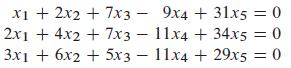
In Problems 15–26, find a basis for the solution space of the given homogeneous linear system. x1 + 2x2 + 7x3 9x4 + 31x5 = 0 2x1 + 4x2 + 7x3 - 11x4 + 34x5: = 0 3x1 + 6x2 + 5x3 - 11x4 + 29x5 = 0
In Problems 12–14, find a basis for the indicated subspace of R4.The set of all vectors of the form (a , b , c , d) for which a + 2b = c + 3d = 0.
In Problems 12–14, find a basis for the indicated subspace of R4.The set of all vectors of the form (a , b , c , d) such that a = 3c and b = 4d.
In Problems 12–14, find a basis for the indicated subspace of R4.The set of all vectors of the form (a , b , c , d) for which a = b + c + d.
In Problems 9–11, find a basis for the indicated subspace of R3.The plane with equation x - 2y + 5z = 0.
In Problems 1–8, determine whether or not the given vectors in Rn form a basis for Rn.v1 = (2 , 0 , 0 , 0) , v2 = (0 , 3 , 0 , 0) , v3 = (0 , 0 , 7, 6) , v4 = (0 , 0 , 4 , 5)
In Problems 1–8, determine whether or not the given vectors in Rn form a basis for Rn.v1 = (0 , 0 , 1) , v2 = (7 , 4 , 11) , v3 = (5 , 3 , 13)
In Problems 1–8, determine whether or not the given vectors in Rn form a basis for Rn.v1 = (0 , 0 , 1) , v2 = ( 0, 1 , 2) , v3 = (1 , 2 , 3)
In Problems 1–8, determine whether or not the given vectors in Rn form a basis for Rn.v1 = (0 , 7 , -3), v2 = (0 , 5 , 4), v3 = (0 , 5 , 10)
In Problems 1–8, determine whether or not the given vectors in Rn form a basis for Rn.v1 = (3 . -7 , 5 , 2) , v2 = (1 , -1 , 3 , 4 ) , v3 = (7 , 11 , 3 , 13)
Showing 900 - 1000
of 2513
First
3
4
5
6
7
8
9
10
11
12
13
14
15
16
17
Last
Step by Step Answers