New Semester Started Get 50% OFF Study Help! --h --m --s Claim Now

Question Answers

Textbooks

Find textbooks, questions and answers

Oops, something went wrong!

Change your search query and then try again

Result Not Found

Books FREE
Study Help
Tutors
AI Study Planner NEW
Sell Books

Search
Sign In
Register

study help
mathematics
first course differential equations

Differential Equations And Linear Algebra 4th Edition C. Edwards, David Penney, David Calvis - Solutions

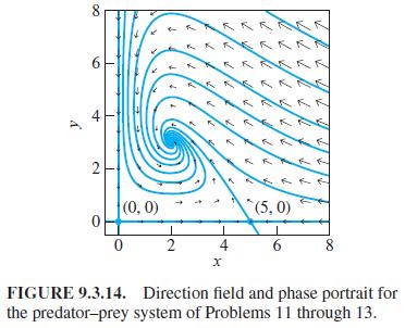
Problems 11 through 13 deal with the predator–prey systemin which the prey population x (t) is logistic but the predator population y(t) would (in the absence of any prey) decline naturally. Problems 11 through 13 imply that the three critical points (0,0), (5,0), and (2,3) of the system in (4)
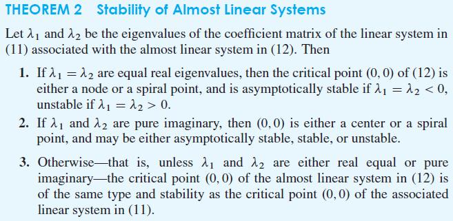
Each of the systems in Problems 11 through 18 has a single critical point (x0 , y0). Apply Theorem 2 to classify this critical point as to type and stability. Verify your conclusion by using a computer system or graphing calculator to construct a phase portrait for the given system.
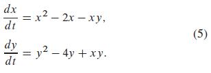
In each of Problems 12 through 16, a second-order equation of the form x'' + f (x, x') = 0, corresponding to a certain mass-and-spring system, is given. Find and classify the critical points of the equivalent first-order system.x'' + 20x - 5x3 = 0: Verify that the critical points resemble those
In Problems 9 through 12, find each equilibrium solution x(t) Ξ x0 of the given second-order differential equation x" + f(x , x') = 0. Use a computer system or graphing calculator to construct a phase portrait and direction field for the equivalent first-order system x' = y, y' = -f(x , y).
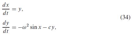
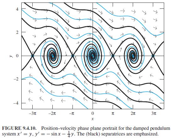
Problems 9 through 11 deal with the damped pendulum system x' = y, y' = -ω2 sinx - cy.Show that if n is an even integer and c2 > 4ω2, then the critical point (nπ, 0) is a spiral sink for the damped pendulum system.
Problems 11 through 13 deal with the predator–prey systemin which the prey population x (t) is logistic but the predator population y(t) would (in the absence of any prey) decline naturally. Problems 11 through 13 imply that the three critical points (0,0), (5,0), and (2,3) of the system in (4)
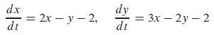
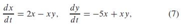
Each of the systems in Problems 11 through 18 has a single critical point (x0 , y0). Apply Theorem 2 to classify this critical point as to type and stability. Verify your conclusion by using a computer system or graphing calculator to construct a phase portrait for the given system. dx dt = 2x - y
In each of Problems 12 through 16, a second-order equation of the form x'' + f (x, x') = 0, corresponding to a certain mass-and-spring system, is given. Find and classify the critical points of the equivalent first-order system.x'' + 2x' + 20x - 5x3 = 0: Verify that the critical points resemble
Problems 11 through 13 deal with the predator–prey systemin which the prey population x (t) is logistic but the predator population y(t) would (in the absence of any prey) decline naturally. Problems 11 through 13 imply that the three critical points (0,0), (5,0), and (2,3) of the system in (4)
In Problems 9 through 12, find each equilibrium solution x(t) Ξ x0 of the given second-order differential equation x" + f(x , x') = 0. Use a computer system or graphing calculator to construct a phase portrait and direction field for the equivalent first-order system x' = y, y' = -f(x , y).
Solve each of the linear systems in Problems 13 through 20 to determine whether the critical point (0, 0) is stable, asymptotically stable, or unstable. Use a computer system or graphing calculator to construct a phase portrait and direction field for the given system. Thereby ascertain the
Each of the systems in Problems 11 through 18 has a single critical point (x0 , y0). Apply Theorem 2 to classify this critical point as to type and stability. Verify your conclusion by using a computer system or graphing calculator to construct a phase portrait for the given system. dx dt = x + y
In each of Problems 12 through 16, a second-order equation of the form x'' + f (x, x') = 0, corresponding to a certain mass-and-spring system, is given. Find and classify the critical points of the equivalent first-order system.x'' - 8x + 2x3 = 0: Here the linear part of the force is repulsive
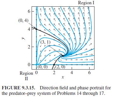
Problems 14 through 17 deal with the predator–prey systemHere each population-the prey population x(t) and the predator population y(t)-is an unsophisticated population (like the alligators of Section 2.1) for which the only alternatives (in the absence of the other population) are doomsday and
Solve each of the linear systems in Problems 13 through 20 to determine whether the critical point (0, 0) is stable, asymptotically stable, or unstable. Use a computer system or graphing calculator to construct a phase portrait and direction field for the given system. Thereby ascertain the
Each of the systems in Problems 11 through 18 has a single critical point (x0 , y0). Apply Theorem 2 to classify this critical point as to type and stability. Verify your conclusion by using a computer system or graphing calculator to construct a phase portrait for the given system. dx dt = x -
In each of Problems 12 through 16, a second-order equation of the form x'' + f (x, x') = 0, corresponding to a certain mass-and-spring system, is given. Find and classify the critical points of the equivalent first-order system.x'' + 4x - x2 = 0: Here the force function is nonsymmetric. Verify that
Solve each of the linear systems in Problems 13 through 20 to determine whether the critical point (0, 0) is stable, asymptotically stable, or unstable. Use a computer system or graphing calculator to construct a phase portrait and direction field for the given system. Thereby ascertain the
Each of the systems in Problems 11 through 18 has a single critical point (x0 , y0). Apply Theorem 2 to classify this critical point as to type and stability. Verify your conclusion by using a computer system or graphing calculator to construct a phase portrait for the given system. dx dt = x - 2y
Problems 14 through 17 deal with the predator–prey systemHere each population-the prey population x(t) and the predator population y(t)-is an unsophisticated population (like the alligators of Section 2.1) for which the only alternatives (in the absence of the other population) are doomsday and
In each of Problems 12 through 16, a second-order equation of the form x'' + f (x, x') = 0, corresponding to a certain mass-and-spring system, is given. Find and classify the critical points of the equivalent first-order system.x'' + 4x - 5x3 + x5 = 0: The idea here is that terms through the fifth
Solve each of the linear systems in Problems 13 through 20 to determine whether the critical point (0, 0) is stable, asymptotically stable, or unstable. Use a computer system or graphing calculator to construct a phase portrait and direction field for the given system. Thereby ascertain the
Problems 14 through 17 deal with the predator–prey systemHere each population-the prey population x(t) and the predator population y(t)-is an unsophisticated population (like the alligators of Section 2.1) for which the only alternatives (in the absence of the other population) are doomsday and
Each of the systems in Problems 11 through 18 has a single critical point (x0 , y0). Apply Theorem 2 to classify this critical point as to type and stability. Verify your conclusion by using a computer system or graphing calculator to construct a phase portrait for the given system. dx dt = x -
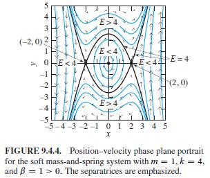
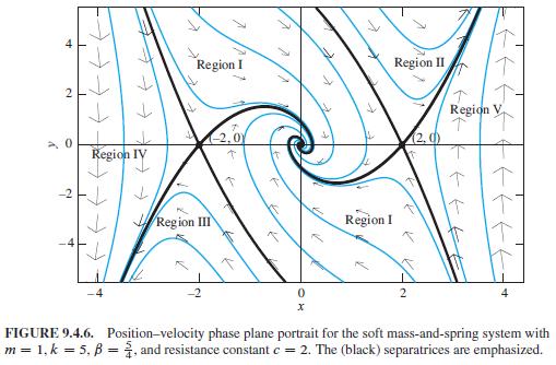
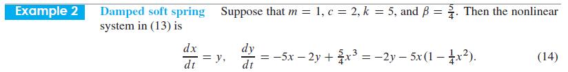
In Problems 17 through 20, analyze the critical points of the indicated system, use a computer system to construct an illustrative position–velocity phase plane portrait, and describe the oscillations that occur.Example 2 in this section illustrates the case of damped vibrations of a soft
Solve each of the linear systems in Problems 13 through 20 to determine whether the critical point (0, 0) is stable, asymptotically stable, or unstable. Use a computer system or graphing calculator to construct a phase portrait and direction field for the given system. Thereby ascertain the
Problems 14 through 17 deal with the predator–prey systemHere each population-the prey population x(t) and the predator population y(t)-is an unsophisticated population (like the alligators of Section 2.1) for which the only alternatives (in the absence of the other population) are doomsday and
Each of the systems in Problems 11 through 18 has a single critical point (x0 , y0). Apply Theorem 2 to classify this critical point as to type and stability. Verify your conclusion by using a computer system or graphing calculator to construct a phase portrait for the given system. dx dt 4x - 5y
In Problems 11 through 14, use the method of Example 4 to find two linearly independent power series solutions of the given differential equation. Determine the radius of convergence of each series, and identify the general solution in terms of familiar elementary functions.y'' + y = x Example
Use the method of Example 6 to find two linearly independent Frobenius series solutions of the differential equations in Problems 27 through 31. Then construct a graph showing their graphs for x > 0.xy" + 2y' + 9xy = 0 Example 6 Find the Frobenius series solutions of xy" + 2y + xy = 0. (31)
In Problems 23 through 26, find a three-term recurrence relation for solutions of the form y = Σ cnxn. Then find the first three nonzero terms in each of two linearly independent solutions.(1 + x3) y'' + x4 y = 0
Solve the initial value problemDetermine sufficiently many terms to compute y(1/2) accurate to four decimal places. y" + xy' + (2x² + 1)y=0; y(0) = 1, y'(0) = -1.
Use the method of Example 6 to find two linearly independent Frobenius series solutions of the differential equations in Problems 27 through 31. Then construct a graph showing their graphs for x > 0.xy" + 2y' - 4xy = 0 Example 6 Find the Frobenius series solutions of xy" + 2y + xy = 0. (31)
In Problems 19 through 30, express the general solution of the given differential equation in terms of Bessel functions.16x2y" - (5 - 144x3) y = 0
Use the method of Example 6 to find two linearly independent Frobenius series solutions of the differential equations in Problems 27 through 31. Then construct a graph showing their graphs for x > 0.4xy" + 8y' + xy = 0 Example 6 Find the Frobenius series solutions of xy" + 2y + xy = 0. (31)
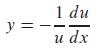
(a) Show that the substitutiontransforms the Riccati equation dy/dx = x2 + y2 into u" + x2u = 0.(b) Show that the general solution of dy/dx = x2 + y2 isApply the identities in Eqs. (22) and (23). 1 du u dx y = --
In Problems 19 through 30, express the general solution of the given differential equation in terms of Bessel functions.2x2y" - 3xy' - 2(14 - x5)y = 0
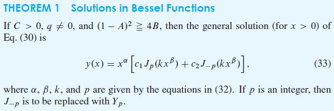
Apply Theorem 1 to show that the general solution ofis y(x) = x-1(A cos x + B sin x). xy" + 2y + xy = 0
In Problems 28 through 30, find the first three nonzero terms in each of two linearly independent solutions of the form y = Σ cnxn. Substitute known Taylor series for the analytic functions and retain enough terms to compute the necessary coefficients.y'' + e-x y = 0
In Problems 19 through 30, express the general solution of the given differential equation in terms of Bessel functions.y'' + x4 y = 0
Use the method of Example 6 to find two linearly independent Frobenius series solutions of the differential equations in Problems 27 through 31. Then construct a graph showing their graphs for x > 0.xy" - y' + 4x3y = 0 Example 6 Find the Frobenius series solutions of xy" + 2y + xy = 0. (31)
In Problems 28 through 30, find the first three nonzero terms in each of two linearly independent solutions of the form y = Σ cnxn. Substitute known Taylor series for the analytic functions and retain enough terms to compute the necessary coefficients.(cos x) y'' + y = 0
Use the method of Example 6 to find two linearly independent Frobenius series solutions of the differential equations in Problems 27 through 31. Then construct a graph showing their graphs for x > 0.4x2y" - 4xy' + (3 - 4x2) y = 0 Example 6 Find the Frobenius series solutions of xy" + 2y + xy =
In Problems 28 through 30, find the first three nonzero terms in each of two linearly independent solutions of the form y = Σ cnxn. Substitute known Taylor series for the analytic functions and retain enough terms to compute the necessary coefficients.xy'' + (sin x) y' + xy = 0
In Problems 19 through 30, express the general solution of the given differential equation in terms of Bessel functions.y" + 4x3 y = 0
Verify that the substitutions in (2) in Bessel’s equation [Eq. (1)] yield Eq. (3). x²y" + xy + (x² - p²) y = 0. (1)
In Problems 32 through 34, find the first three nonzero terms of each of two linearly independent Frobenius series solutions.2x2y" + x(x + 1)y' - (2x + 1)y = 0
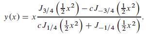
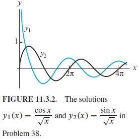
Apply the method of Frobenius to Bessel’s equation of order 1/2,to derive its general solution for x > 0,Figure 11.3.2 shows the graphs of the two indicated solutions. x²y" + xy + (x² - 1) y = 0,
Note that x = 0 is an irregular point of the equation(a) Show that y = xr Σ cnxn can satisfy this equation only if r = 0.(b) Substitute y = Σ cnxn to derive the "formal" solution y = Σ n!xn. What is the radius of con- vergence of this series? x²y" + (3x - 1)y' + y = 0.
In Problems 32 through 34, find the first three nonzero terms of each of two linearly independent Frobenius series solutions.(2x2 + 5x3)y" + (3x - x2)y' - (1 + x) y = 0
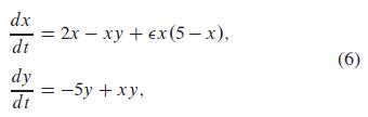
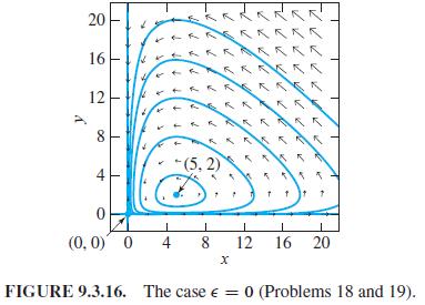
Problems 18 through 25 deal with the predator–prey systemfor which a bifurcation occurs at the value ∈ = 0 of the parameter ∈ . Problems 18 and 19 deal with the case ∈ = 0, in which case the system in (6) takes the formand these problems suggest that the two critical points (0,0) and (5,2)
(a) Suppose that A and B are nonzero constants. Show that the equation x2y" + Ay' + By = 0 has at most one solution of the form y = xr Σcnxn.(b) Repeat part (a) with the equation x3y" + Axy' + By = 0.(c) Show that the equation x3y" + Ax2y' + By = 0 has no Frobenius series solution.
In Problems 32 through 34, find the first three nonzero terms of each of two linearly independent Frobenius series solutions.2x2y'' + (sin x)y' - (cos x)y = 0
Solve each of the linear systems in Problems 13 through 20 to determine whether the critical point (0, 0) is stable, asymptotically stable, or unstable. Use a computer system or graphing calculator to construct a phase portrait and direction field for the given system. Thereby ascertain the
Problems 18 through 25 deal with the predator–prey systemfor which a bifurcation occurs at the value ∈ = 0 of the parameter ∈ . Problems 18 and 19 deal with the case ∈ = 0, in which case the system in (6) takes the formand these problems suggest that the two critical points (0,0) and (5,2)
In Problems 17 through 20, analyze the critical points of the indicated system, use a computer system to construct an illustrative position–velocity phase plane portrait, and describe the oscillations that occur.Now repeat Example 2 with both the alterations corresponding to Problems 17 and 18.
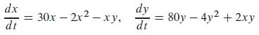
In Problems 19 through 28, investigate the type of the critical point (0 , 0) of the given almost linear system. Verify your conclusion by using a computer system or graphing calculator to construct a phase portrait. Also, describe the approximate locations and apparent types of any other critical
In Problems 17 through 20, analyze the critical points of the indicated system, use a computer system to construct an illustrative position–velocity phase plane portrait, and describe the oscillations that occur.The equations x' = y, y' = -sin x - 1/4 y |y| model a damped pendulum system as in
In Problems 19 through 28, investigate the type of the critical point (0 , 0) of the given almost linear system. Verify your conclusion by using a computer system or graphing calculator to construct a phase portrait. Also, describe the approximate locations and apparent types of any other critical
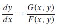
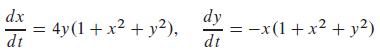
In Problems 23 through 26, a system dx/dt = F(x, y), dy/dt = G(x, y) is given. Solve the equationto find the trajectories of the given system. Use a computer systemor graphing calculator to construct a phase portrait and direction field for the system, and thereby identify visually the apparent
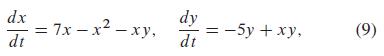
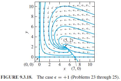
Problems 23 through 25 deal with the case ∈ = 1, so that the system in (6) takes the formand these problems imply that the three critical points (0,0), (7,0), and (5,2) of the system in (9) are as shown in Fig. 9.3.18 -with saddle points at the origin and on the positive x-axis and with a spiral
In Problems 19 through 28, investigate the type of the critical point (0 , 0) of the given almost linear system. Verify your conclusion by using a computer system or graphing calculator to construct a phase portrait. Also, describe the approximate locations and apparent types of any other critical
The term bifurcation generally refers to something “splitting apart.” With regard to differential equations or systems involving a parameter, it refers to abrupt changes in the character of the solutions as the parameter is changed continuously. Problems 33 through 36 illustrate sensitive cases
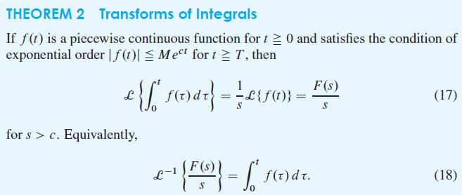
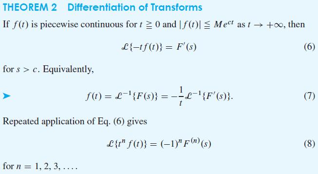
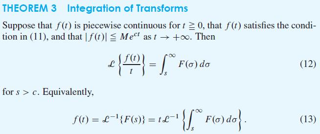
In Problems 15 through 22, apply either Theorem 2 or Theorem 3 to find the Laplace transform of f (t). f(t)= = 1 - cos 2t t
Apply Theorem 2 to find the inverse Laplace transforms of the functions in Problems 17 through 24. F(s) = 1 s² (s² + 1)
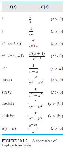
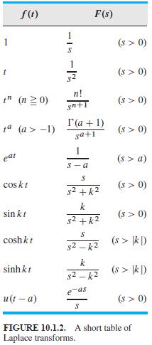
Use the transforms in Fig. 10.1.2 to find the Laplace transforms of the functions in Problems 11 through 22. A preliminary integration by parts may be necessary. f (t) = t cos 2t t f(t) t" (n ≥ 0) ta (a> -1) eat coskt sin kt cosh kt sinhkt u(t - a) S n! gn+T F(s) I (a +
In Problems 15 through 22, apply either Theorem 2 or Theorem 3 to find the Laplace transform of f (t). f(t) = et - e-t t
Use the transforms in Fig. 10.1.2 to find the Laplace transforms of the functions in Problems 11 through 22. A preliminary integration by parts may be necessary. f (t) = sinh2 3t t f(t) t" (n ≥0) g@ (a>−1) eat cos kt sin kt cosh kt sinhkt u(t - a) 13 S n! gn+T F(s) Γ(α +
Solve each of the linear systems in Problems 13 through 20 to determine whether the critical point (0, 0) is stable, asymptotically stable, or unstable. Use a computer system or graphing calculator to construct a phase portrait and direction field for the given system. Thereby ascertain the
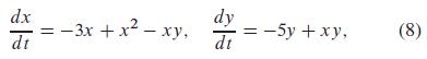
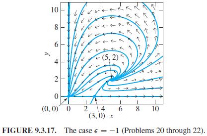
Problems 20 through 22 deal with the case ∈ = -1, for which the system in (6) becomesand imply that the three critical points (0,0), (3,0), and (5,2) of (8) are as shown in Fig. 9.3.17-with a nodal sink at the origin, a saddle point on the positive x-axis, and a spiral source at (5,2). In each
In Problems 19 through 28, investigate the type of the critical point (0 , 0) of the given almost linear system. Verify your conclusion by using a computer system or graphing calculator to construct a phase portrait. Also, describe the approximate locations and apparent types of any other critical
Solve each of the linear systems in Problems 13 through 20 to determine whether the critical point (0, 0) is stable, asymptotically stable, or unstable. Use a computer system or graphing calculator to construct a phase portrait and direction field for the given system. Thereby ascertain the
Problems 20 through 22 deal with the case ∈ = -1, for which the system in (6) becomesand imply that the three critical points (0,0), (3,0), and (5,2) of (8) are as shown in Fig. 9.3.17-with a nodal sink at the origin, a saddle point on the positive x-axis, and a spiral source at (5,2). In each
In Problems 19 through 28, investigate the type of the critical point (0 , 0) of the given almost linear system. Verify your conclusion by using a computer system or graphing calculator to construct a phase portrait. Also, describe the approximate locations and apparent types of any other critical
Problems 20 through 22 deal with the case ∈ = -1, for which the system in (6) becomesand imply that the three critical points (0,0), (3,0), and (5,2) of (8) are as shown in Fig. 9.3.17-with a nodal sink at the origin, a saddle point on the positive x-axis, and a spiral source at (5,2). In each
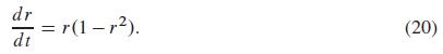
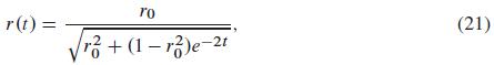
Separate variables in Eq. (20) to derive the solution in (21). dr dt =r(1-²). (20)
In Problems 23 through 26, a system dx/dt = F(x, y), dy/dt = G(x, y) is given. Solve the equationto find the trajectories of the given system. Use a computer system or graphing calculator to construct a phase portrait and direction field for the system, and thereby identify visually the apparent
In Problems 19 through 28, investigate the type of the critical point (0, 0) of the given almost linear system. Verify your conclusion by using a computer system or graphing calculator to construct a phase portrait. Also, describe the approximate locations and apparent types of any other critical
Problems 23 through 25 deal with the case ∈ = 1, so that the system in (6) takes the formand these problems imply that the three critical points (0,0), (7,0), and (5,2) of the system in (9) are as shown in Fig. 9.3.18 -with saddle points at the origin and on the positive x-axis and with a spiral
In Problems 23 through 26, a system dx/dt = F(x, y), dy/dt = G(x, y) is given. Solve the equationto find the trajectories of the given system. Use a computer systemor graphing calculator to construct a phase portrait and direction field for the system, and thereby identify visually the apparent
Problems 23 through 25 deal with the case ∈ = 1, so that the system in (6) takes the formand these problems imply that the three critical points (0,0), (7,0), and (5,2) of the system in (9) are as shown in Fig. 9.3.18 -with saddle points at the origin and on the positive x-axis and with a spiral
In Problems 23 through 26, a system dx/dt = F(x, y), dy/dt = G(x, y) is given. Solve the equationto find the trajectories of the given system. Use a computer systemor graphing calculator to construct a phase portrait and direction field for the system, and thereby identify visually the apparent
In Problems 19 through 28, investigate the type of the critical point (0 , 0) of the given almost linear system. Verify your conclusion by using a computer system or graphing calculator to construct a phase portrait. Also, describe the approximate locations and apparent types of any other critical
In Problems 19 through 28, investigate the type of the critical point (0 , 0) of the given almost linear system. Verify your conclusion by using a computer system or graphing calculator to construct a phase portrait. Also, describe the approximate locations and apparent types of any other critical
For each two-population system in Problems 26 through 34, first describe the type of x- and y-populations involved (exponential or logistic) and the nature of their interaction— competition, cooperation, or predation. Then find and characterize the system’s critical points (as to type and
In Problems 19 through 28, investigate the type of the critical point (0 , 0) of the given almost linear system. Verify your conclusion by using a computer system or graphing calculator to construct a phase portrait. Also, describe the approximate locations and apparent types of any other critical
For each two-population system in Problems 26 through 34, first describe the type of x- and y-populations involved (exponential or logistic) and the nature of their interaction— competition, cooperation, or predation. Then find and characterize the system’s critical points (as to type and
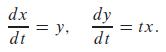
Let (x(t) , y(t)) be a nontrivial solution of the nonautonomous systemSuppose that ϕ(t) = x (t + ϒ) and Ψ(t) = y(t + ϒ), where y ≠ 0. Show that (ϕ(t), Ψ (t)) is not a solution of the system. dx 15 dt = y. dy dt = tx.
For each two-population system in Problems 26 through 34, first describe the type of x- and y-populations involved (exponential or logistic) and the nature of their interaction— competition, cooperation, or predation. Then find and characterize the system’s critical points (as to type and
In Problems 19 through 28, investigate the type of the critical point (0 , 0) of the given almost linear system. Verify your conclusion by using a computer system or graphing calculator to construct a phase portrait. Also, describe the approximate locations and apparent types of any other critical
For each two-population system in Problems 26 through 34, first describe the type of x- and y-populations involved (exponential or logistic) and the nature of their interaction— competition, cooperation, or predation. Then find and characterize the system’s critical points (as to type and
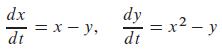
In Problems 29 through 32, find all critical points of the given system, and investigate the type and stability of each. Verify your conclusions by means of a phase portrait constructed using a computer system or graphing calculator. dx dt = x - y, dy dt =x²-y
For each two-population system in Problems 26 through 34, first describe the type of x- and y-populations involved (exponential or logistic) and the nature of their interaction— competition, cooperation, or predation. Then find and characterize the system’s critical points (as to type and
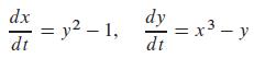
In Problems 29 through 32, find all critical points of the given system, and investigate the type and stability of each. Verify your conclusions by means of a phase portrait constructed using a computer system or graphing calculator. dx dt = y - 1, dx = x² - y dy dt
For each two-population system in Problems 26 through 34, first describe the type of x-and y-populations involved (exponential or logistic) and the nature of their interaction— competition, cooperation, or predation. Then find and characterize the system’s critical points (as to type and
For each two-population system in Problems 26 through 34, first describe the type of x-and y-populations involved (exponential or logistic) and the nature of their interaction— competition, cooperation, or predation. Then find and characterize the system’s critical points (as to type and
In Problems 29 through 32, find all critical points of the given system, and investigate the type and stability of each. Verify your conclusions by means of a phase portrait constructed using a computer system or graphing calculator. dx dt = y2 - 1, dy = dt = x³ - у — у
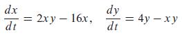
In Problems 29 through 32, find all critical points of the given system, and investigate the type and stability of each. Verify your conclusions by means of a phase portrait constructed using a computer system or graphing calculator. dx dt = xy - 2, dy dt = x - 2y
For each two-population system in Problems 26 through 34, first describe the type of x- and y-populations involved (exponential or logistic) and the nature of their interaction— competition, cooperation, or predation. Then find and characterize the system’s critical points (as to type and
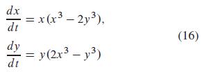
In the case of a two-dimensional system that is not almost linear, the trajectories near an isolated critical point can exhibit a considerably more complicated structure than those near the nodes, centers, saddle points, and spiral points discussed in this section. For example, consider the

Showing 400 - 500 of 2513

1
2
3
4
5
6
7
8
9
10
11
12
13
14
15
Last

Step by Step Answers

Services

Sitemap
Fun
Definitions
Become Tutor
Used Textbooks
Study Help Categories
Recent Questions
Expert Questions
Campus Wear
Sell Your Books

Company Info

Security
Copyrights
Privacy Policy
Terms & Conditions
SolutionInn Fee
Scholarship
Online Quiz
Give Feedback, Get Rewards

Get In Touch

About Us
Contact Us
Career
Jobs
FAQ
Student Discount
Campus Ambassador

Secure Payment

Download Our App

© 2026 SolutionInn. All Rights Reserved