New Semester
Started
Get
50% OFF
Study Help!
--h --m --s
Claim Now
Question Answers
Textbooks
Find textbooks, questions and answers
Oops, something went wrong!
Change your search query and then try again
S
Books
FREE
Study Help
Expert Questions
Accounting
General Management
Mathematics
Finance
Organizational Behaviour
Law
Physics
Operating System
Management Leadership
Sociology
Programming
Marketing
Database
Computer Network
Economics
Textbooks Solutions
Accounting
Managerial Accounting
Management Leadership
Cost Accounting
Statistics
Business Law
Corporate Finance
Finance
Economics
Auditing
Tutors
Online Tutors
Find a Tutor
Hire a Tutor
Become a Tutor
AI Tutor
AI Study Planner
NEW
Sell Books
Search
Search
Sign In
Register
study help
mathematics
first course differential equations
Differential Equations And Linear Algebra 4th Edition C. Edwards, David Penney, David Calvis - Solutions
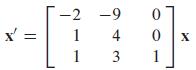
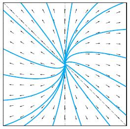
Find general solutions of the systems in Problems 1 through 22. In Problems 1 through 6, use a computer system or graphing calculator to construct a direction field and typical solution curves for the given system. X' -2 1 1 -9 4 3 0 0 1 X
In Problems 13 through 22, first verify that the given vectors are solutions of the given system. Then use the Wronskian to show that they are linearly independent. Finally, write the general solution of the system. - 1 x = [ 3₂ ] } ] × × = ²² [ } ]- x₂ = c ² [ ] x' X; X1 e²t 5 -3 X2 e-2t
Use the method of Examples 5, 6, and 7 to find general solutions of the systems in Problems 11 through 20. If initial conditions are given, find the corresponding particular solution. For each problem, use a computer system or graphing calculator to construct a direction field and typical solution
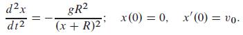
Suppose that a projectile is fired straight upward with initial velocity v0 from the surface of the earth. If air resistance is not a factor, then its height x(t) at time t satisfies the initial value problemUse the values g = 32.15 ft/s2 ≈ 0.006089 mi/s2 for the gravitational acceleration
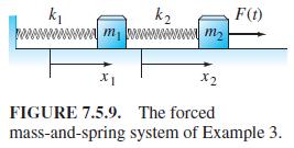
Suppose that m1 = 2, m2 = 1/2, k1 = 75, k2 = 25, F0 = 100, and ω = 10 (all in mks units) in the forced mass-and- spring system of Fig. 7.5.9. Find the solution of the system Mx" = Kx + F that satisfies the initial conditions x(0) = x'(0) = 0. k₁ k₂ www.m
In Problems 1 through 16, apply the eigenvalue method of this section to find a general solution of the given system. If initial values are given, find also the corresponding particular solution. For each problem, use a computer system or graphing calculator to construct a direction field and
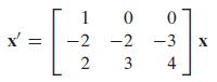
Find general solutions of the systems in Problems 1 through 22. In Problems 1 through 6, use a computer system or graphing calculator to construct a direction field and typical solution curves for the given system. 10 = -2 -2 -2 3 NN 2 0 -3 4 X
Use the method of Examples 5, 6, and 7 to find general solutions of the systems in Problems 11 through 20. If initial conditions are given, find the corresponding particular solution. For each problem, use a computer system or graphing calculator to construct a direction field and typical solution
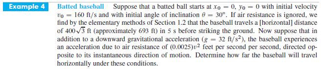
Problems 16 through 18 deal with the batted baseball of Example 4, having initial velocity 160 ft/s and air resistance coefficient c = 0.0025.Find the range—the horizontal distance the ball travels before it hits the ground—and its total time of flight with initial inclination angles 40°,
In Problems 13 through 22, first verify that the given vectors are solutions of the given system. Then use the Wronskian to show that they are linearly independent. Finally, write the general solution of the system. 1 x = [ ₁² ]x²x₁ = e³²¹ [ _ 1] x₂ = ²² [-₂] -2 X; e3t X2 e²t
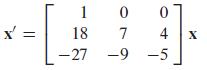
Find general solutions of the systems in Problems 1 through 22. In Problems 1 through 6, use a computer system or graphing calculator to construct a direction field and typical solution curves for the given system. X 1 18 -27 -9 -5 0 0 7 4 45 X
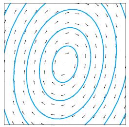
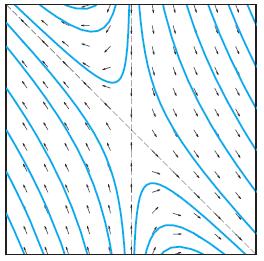
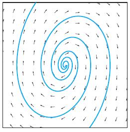
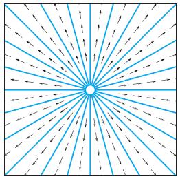
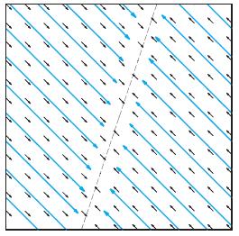
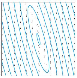
The phase portraits in Problems 17 through 28 correspond to linear systems of the form x' = Ax in which the matrix A has two linearly independent eigenvectors. Determine the nature of the eigenvalues and eigenvectors of each system. For example, you may discern that the system has pure imaginary
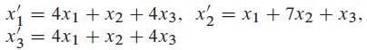
In Problems 17 through 25, the eigenvalues of the coefficient matrix can be found by inspection and factoring. Apply the eigenvalue method to find a general solution of each system. | = 4x1 + x2 + 4x3, x₂ = x₁ +7x2 + x3, x3 = 4x1 + x2 + 4x3
Problems 16 through 18 deal with the batted baseball of Example 4, having initial velocity 160 ft/s and air resistance coefficient c = 0.0025.Find (to the nearest degree) the initial inclination that maximizes the range. If there were no air resistance it would be exactly 45°, but your answer
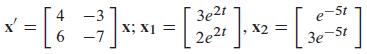
In Problems 13 through 22, first verify that the given vectors are solutions of the given system. Then use the Wronskian to show that they are linearly independent. Finally, write the general solution of the system. 4-3 x = [6 =]× × = [2²]- x2 = [ 3e21 X; -7 X2 2e2t e-St St Зе-5
Use the method of Examples 5, 6, and 7 to find general solutions of the systems in Problems 11 through 20. If initial conditions are given, find the corresponding particular solution. For each problem, use a computer system or graphing calculator to construct a direction field and typical solution
The phase portraits in Problems 17 through 28 correspond to linear systems of the form x' = Ax in which the matrix A has two linearly independent eigenvectors. Determine the nature of the eigenvalues and eigenvectors of each system. For example, you may discern that the system has pure imaginary
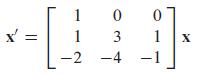
Find general solutions of the systems in Problems 1 through 22. In Problems 1 through 6, use a computer system or graphing calculator to construct a direction field and typical solution curves for the given system. = 10 1 3 -4 -2 0 1 -1 X
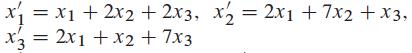
In Problems 17 through 25, the eigenvalues of the coefficient matrix can be found by inspection and factoring. Apply the eigenvalue method to find a general solution of each system. x1 = x1 + 2x2 + 2x3, x2 = 2x1 +7x2 + x3, x3 = 2x1 + x2 +7x3
Use the method of Examples 5, 6, and 7 to find general solutions of the systems in Problems 11 through 20. If initial conditions are given, find the corresponding particular solution. For each problem, use a computer system or graphing calculator to construct a direction field and typical solution
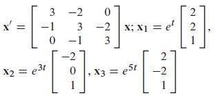
In Problems 13 through 22, first verify that the given vectors are solutions of the given system. Then use the Wronskian to show that they are linearly independent. Finally, write the general solution of the system. x = [- 3 -1 0-1 -2 0 2 32 X; X1 = e¹|| 2 3 [H] 0 , X3 = e5t -2 1 X2 = e3t 2
Problems 16 through 18 deal with the batted baseball of Example 4, having initial velocity 160 ft/s and air resistance coefficient c = 0.0025.Find (to the nearest half degree) the initial inclination angle greater than 45° for which the range is 300 ft. Example 4 Batted baseball Suppose that a
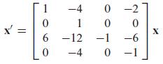
Find general solutions of the systems in Problems 1 through 22. In Problems 1 through 6, use a computer system or graphing calculator to construct a direction field and typical solution curves for the given system. X' 1 0 6 -12 0 -4 -4 1 0-2 0 0 -1 -6 0 -1 X
The phase portraits in Problems 17 through 28 correspond to linear systems of the form x' = Ax in which the matrix A has two linearly independent eigenvectors. Determine the nature of the eigenvalues and eigenvectors of each system. For example, you may discern that the system has pure imaginary
Use the method of Examples 5, 6, and 7 to find general solutions of the systems in Problems 11 through 20. If initial conditions are given, find the corresponding particular solution. For each problem, use a computer system or graphing calculator to construct a direction field and typical solution
In Problems 17 through 25, the eigenvalues of the coefficient matrix can be found by inspection and factoring. Apply the eigenvalue method to find a general solution of each system. x₁ = 4x₁ + x2 + x3, x2 x1 + x2 + 4x3 = x1 + 4x2 + x3, x3 =
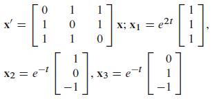
In Problems 13 through 22, first verify that the given vectors are solutions of the given system. Then use the Wronskian to show that they are linearly independent. Finally, write the general solution of the system. X' 0 1 1 0 1 1 1 0 X; X₁ = e2t1 *=~[ - |-~=~[] x2 = e-t X3 e
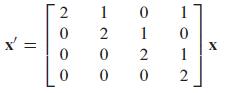
Find general solutions of the systems in Problems 1 through 22. In Problems 1 through 6, use a computer system or graphing calculator to construct a direction field and typical solution curves for the given system. = 2 0 0 0 1 2 0 0 0 0120 1 2 0 1 0 1 2 X
Find the initial velocity of a baseball hit by Babe Ruth (with c = 0.0025 and initial inclination 40°) if it hit the bleachers at a point 50 ft high and 500 horizontal feet from home plate.
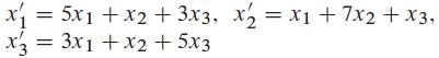
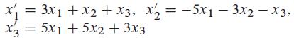
In Problems 17 through 25, the eigenvalues of the coefficient matrix can be found by inspection and factoring. Apply the eigenvalue method to find a general solution of each system. x3 = 5x1 + x2 + 3x3, x₂ = x₁ + 7x₂ + x3, 3x1 + x2 + 5x3
The phase portraits in Problems 17 through 28 correspond to linear systems of the form x' = Ax in which the matrix A has two linearly independent eigenvectors. Determine the nature of the eigenvalues and eigenvectors of each system. For example, you may discern that the system has pure imaginary
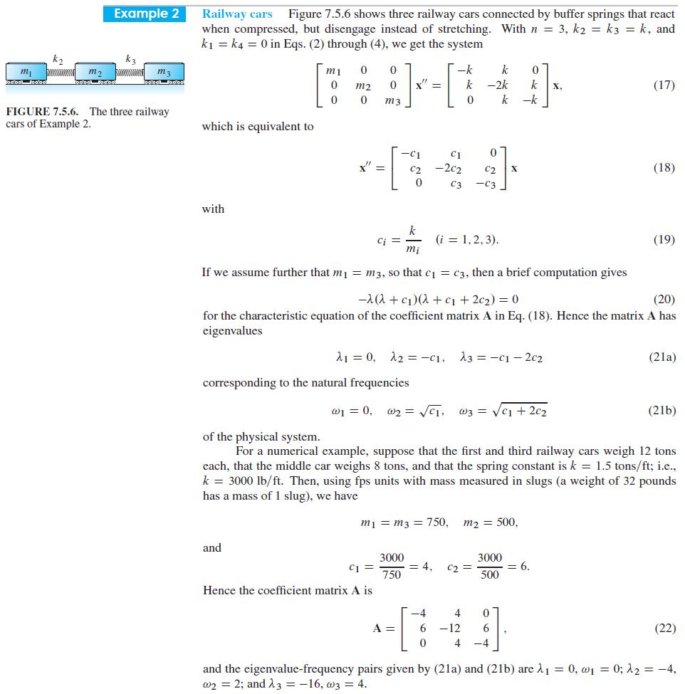
Problems 20 through 23 deal with the same system of three railway cars (same masses) and two buffer springs (same spring constants) as shown in Fig. 7.5.6 and discussed in Example 2. The cars engage at time t = 0 with x1(0) = x2 (0) = x3 (0) = 0 and with the given initial velocities (where v0 = 48
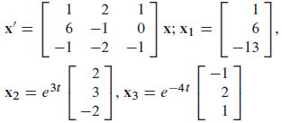
In Problems 13 through 22, first verify that the given vectors are solutions of the given system. Then use the Wronskian to show that they are linearly independent. Finally, write the general solution of the system. -[₁ 1 6 x2 = 31 2 -1 -2 1 0 X; X1 2 [D] 3 X3 = e-4t -2 -1-₁ 1 6 -13 2 1
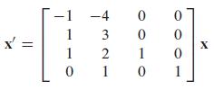
Find general solutions of the systems in Problems 1 through 22. In Problems 1 through 6, use a computer system or graphing calculator to construct a direction field and typical solution curves for the given system. x = -1 -4 1 1 2 0 1 0 3 0 1 0 0 0 0 1 X
Consider the crossbow bolt of Problem 14, fired with the same initial velocity of 288 ft/s and with the air resistance deceleration (0.0002)v2 directed opposite its direction of motion. Suppose that this bolt is fired from ground level at an initial angle of 45°. Find how high vertically and how
In Problems 17 through 25, the eigenvalues of the coefficient matrix can be found by inspection and factoring. Apply the eigenvalue method to find a general solution of each system. x₁ = 5x1-6x3, x₂ = 2x1-x2-2x3, x3 = 4x1-2x2 4x3 -
The phase portraits in Problems 17 through 28 correspond to linear systems of the form x' = Ax in which the matrix A has two linearly independent eigenvectors. Determine the nature of the eigenvalues and eigenvectors of each system. For example, you may discern that the system has pure imaginary
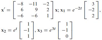
In Problems 13 through 22, first verify that the given vectors are solutions of the given system. Then use the Wronskian to show that they are linearly independent. Finally, write the general solution of the system. -8 6 -6 Xx2 = et -11 9 -6 -2 2 1 X; X1 = e XI e-21 X3 = e3t 3 -2 2
Suppose that an artillery projectile is fired from ground level with initial velocity 3000 ft/s and initial inclination angle 40°. Assume that its air resistance deceleration is (0.0001)v2.(a) What is the range of the projectile and what is its total time of flight? What is its speed at impact
Problems 20 through 23 deal with the same system of three railway cars (same masses) and two buffer springs (same spring constants) as shown in Fig. 7.5.6 and discussed in Example 2. The cars engage at time t = 0 with x1(0) = x2 (0) = x3 (0) = 0 and with the given initial velocities (where v0 = 48
(a) Calculate [x (t)]2 + [y(t)]2 to show that the trajectories of the system x' = y, y' = -x of Problem 11 are circles. (b) Calculate [x (t)]2 - [y(t)]2 to show that the trajectories of the system x' = y, y' = x of Problem 12 are hyperbolas. Problem 11x' = y, y' = -x Problem
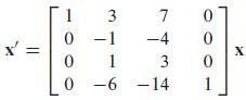
Find general solutions of the systems in Problems 1 through 22. In Problems 1 through 6, use a computer system or graphing calculator to construct a direction field and typical solution curves for the given system. = 1 3 0-1 0 1 9- 0 7 -4 3 -6-14 0 0 0 1 X
The phase portraits in Problems 17 through 28 correspond to linear systems of the form x' = Ax in which the matrix A has two linearly independent eigenvectors. Determine the nature of the eigenvalues and eigenvectors of each system. For example, you may discern that the system has pure imaginary
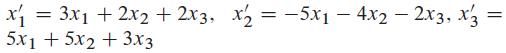
In Problems 17 through 25, the eigenvalues of the coefficient matrix can be found by inspection and factoring. Apply the eigenvalue method to find a general solution of each system. - x₁ = 3x₁ + 2x2 + 2x3, x₂ = −5x₁ − 4x2 − 2x3, x'3 5x1 + 5x2 + 3x3 || =
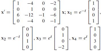
In Problems 13 through 22, first verify that the given vectors are solutions of the given system. Then use the Wronskian to show that they are linearly independent. Finally, write the general solution of the system. x 1 0 0-2 0 0 -6 -1 0 -1 1 [] [] x3 = ef 1 X2 = e-t -4 1 6-12 -4 0 圓 X; x1 =
(a) Beginning with the general solution of the system x' = -2y, y' = 2x of Problem 13, calculate x2 + y2 to show that the trajectories are circles.(b) Show similarly that the trajectories of the system x' = 1/2y, y' = -8x of Problem 15 are ellipses with equations of the form 16x2 + y2 = C2.Problems
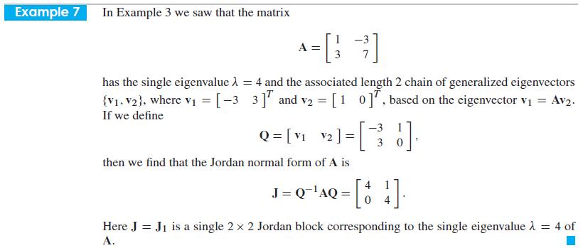
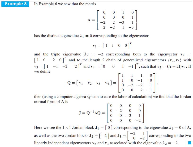
Use the method of Examples 7 and 8 to find the Jordan normal form J of each coefficient matrix A given in Problems 23 through 32 (respectively). Example 7 In Example 3 we saw that the matrix ^=[03] A 7 = has the single eigenvalue > {V₁, V2), where V₁ = [-3 If we define 4 and the associated
Use the method of Examples 7 and 8 to find the Jordan normal form J of each coefficient matrix A given in Problems 23 through 32 (respectively). Example 7 In Example 3 we saw that the matrix ^=[03] A 7 = has the single eigenvalue > {V₁, V2), where V₁ = [-3 If we define 4 and the associated
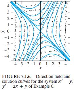
First solve Eqs. (16) and (17) for e-t and e2t in terms of x(t), y(t), and the constants A and B. Then substitute the results in (e2t) (e-t)2 = 1 to show that the trajectories of the system x' = y, y' = 2x + y in Example 6 satisfy an equation of the formThen show that C = 0 yields the straight
Use projection matrices to find a fundamental matrix solution of each of the linear systems given in Problems 1 through 10.m1 = 1 , m2 = 2; k1 = 2 , k2 = k3 = 4
Apply the method of undetermined coefficients to find a particular solution of each of the systems in Problems 1 through 14. If initial conditions are given, find the particular solution that satisfies these conditions. Primes denote derivatives with respect to t.x' = 2x + y + 1, y' = 4x + 2y + e4t
Compute the matrix exponential eAt for each system x' = Ax given in Problems 9 through 20.x'1 = 11x1 - 15x2, x'2 = 6x1 - 8x2
Problems 20 through 23 deal with the same system of three railway cars (same masses) and two buffer springs (same spring constants) as shown in Fig. 7.5.6 and discussed in Example 2. The cars engage at time t = 0 with x1(0) = x2 (0) = x3 (0) = 0 and with the given initial velocities (where v0 = 48
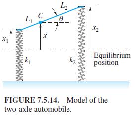
In Problems 27 through 29, the system of Fig. 7.5.14 is taken as a model for an undamped car with the given parameters in fps units. (a) Find the two natural frequencies of oscillation (in hertz). (b) Assume that this car is driven along a sinusoidal washboard surface with a wavelength of 40 ft.
In Problems 23 through 32, find a particular solution of the indicated linear system that satisfies the given initial conditions.The system of Problem 22: x1 (0) = 1, x2 (0) = 3, x3 (0) = 4, x4(0) = 7
The phase portraits in Problems 17 through 28 correspond to linear systems of the form x' = Ax in which the matrix A has two linearly independent eigenvectors. Determine the nature of the eigenvalues and eigenvectors of each system. For example, you may discern that the system has pure imaginary
In Problems 17 through 25, the eigenvalues of the coefficient matrix can be found by inspection and factoring. Apply the eigenvalue method to find a general solution of each system. x₁ = 3x₁ + x₂ + x3, x₂ = -5x₁ - 3x2 - x3, x2 x3 = 5x1 + 5x2 + 3x3
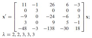
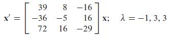
In Problems 23 through 32 the eigenvalues of the coefficient matrix A are given. Find a general solution of the indicated system x' = Ax. Especially in Problems 29 through 32, use of a computer algebra system (as in the application material for this section) may be useful.
In Problems 23 through 32, find a particular solution of the indicated linear system that satisfies the given initial conditions.The system of Problem 14: x1 (0) = 0, x2 (0) = 5
Problems 20 through 23 deal with the same system of three railway cars (same masses) and two buffer springs (same spring constants) as shown in Fig. 7.5.6 and discussed in Example 2. The cars engage at time t = 0 with x1(0) = x2 (0) = x3 (0) = 0 and with the given initial velocities (where v0 = 48
The phase portraits in Problems 17 through 28 correspond to linear systems of the form x' = Ax in which the matrix A has two linearly independent eigenvectors. Determine the nature of the eigenvalues and eigenvectors of each system. For example, you may discern that the system has pure imaginary
In each of Problems 41 through 46, use the spectral decomposition methods of this section to find a fundamental matrix solution x(t) = eAt for the linear system x' = Ax given in the problem.Problem 23 in Section 7.5 x₁ (0) = 3vo, x₂ (0) = 2vo, x3 (0) = 200
Use projection matrices to find a fundamental matrix solution of each of the linear systems given in Problems 1 through 10.The mass-and-spring system of Problem 2, with F1(t) = 96 cos 5t , F2(t) Ξ 0Problem 2m1 = m2 = 1; k1 = 1, k2 = 4, k3 = 1
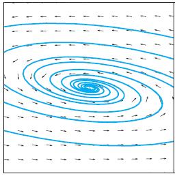
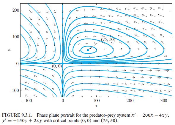
Problems 1 and 2 deal with the predator–prey systemthat corresponds to Fig. 9.3.1.Starting with the Jacobian matrix of the system in (1), derive its linearizations at the two critical points (0 , 0) and (75 , 50). Use a graphing calculator or computer system to construct phase plane portraits for
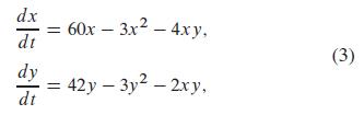
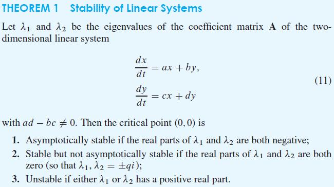
In Problems 1 through 10, apply Theorem 1 to determine the type of the critical point (0 , 0) and whether it is asymptotically stable, stable, or unstable. Verify your conclusion by using a computer system or graphing calculator to construct a phase portrait for the given linear system. dx dt -2x +
Problems 1 and 2 deal with the predator–prey systemthat corresponds to Fig. 9.3.1.Separate the variables in the quotientof the two equations in (1), and thereby derive the exact implicit solutionof the system. Use the contour plot facility of a graphing calculator or computer system to plot the
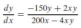
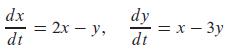
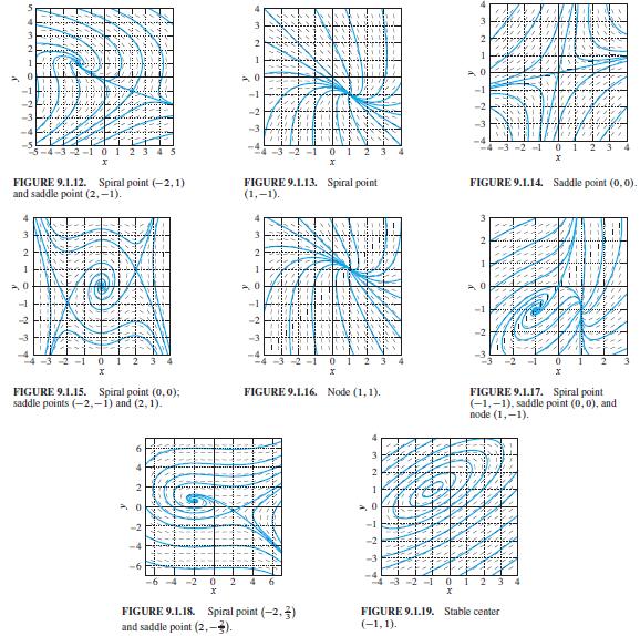
In Problems 1 through 8, find the critical point or points of the given autonomous system, and thereby match each system with its phase portrait among Figs. 9.1.12 through 9.1.19. dx dt = 2x - y, dy dt = x - 3y
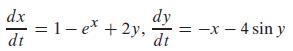
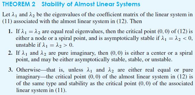
In Problems 1 through 4, show that the given system is almost linear with (0 , 0) as a critical point, and classify this critical point as to type and stability. Use a computer system or graphing calculator to construct a phase plane portrait that illustrates your conclusion. dx dt = 1-e* + 2y, =
In Problems 1 through 10, apply Theorem 1 to determine the type of the critical point (0 , 0) and whether it is asymptotically stable, stable, or unstable. Verify your conclusion by using a computer system or graphing calculator to construct a phase portrait for the given linear system. dx dt = 4x
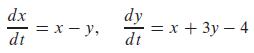
In Problems 1 through 8, find the critical point or points of the given autonomous system, and thereby match each system with its phase portrait among Figs. 9.1.12 through 9.1.19. dx dt = x - y, dy dt = x + 3y - 4
In Problems 1 through 4, show that the given system is almost linear with (0, 0) as a critical point, and classify this critical point as to type and stability. Use a computer system or graphing calculator to construct a phase plane portrait that illustrates your conclusion. dx dt 2 sin x + sin
In Problems 1 through 10, apply Theorem 1 to determine the type of the critical point (0 , 0) and whether it is asymptotically stable, stable, or unstable. Verify your conclusion by using a computer system or graphing calculator to construct a phase portrait for the given linear system. dx dt = x +
Let x(t) be a harmful insect population (aphids?) that under natural conditions is held somewhat in check by a benign predator insect population y(t) (ladybugs?). Assume that x(t) and y(t) satisfy the predator–prey equations in (1), so that the stable equilibrium populations are xE = b/q and yE =
In Problems 1 through 4, show that the given system is almost linear with (0 , 0) as a critical point, and classify this critical point as to type and stability. Use a computer system or graphing calculator to construct a phase plane portrait that illustrates your conclusion. dx dt = ex + 2y -
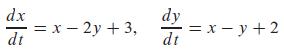
In Problems 1 through 8, find the critical point or points of the given autonomous system, and thereby match each system with its phase portrait among Figs. 9.1.12 through 9.1.19. dx dt = x - 2y + 3, dy dt = x - y +2
In Problems 1 through 10, apply Theorem 1 to determine the type of the critical point (0 , 0) and whether it is asymptotically stable, stable, or unstable. Verify your conclusion by using a computer system or graphing calculator to construct a phase portrait for the given linear system. dx dt = 3x
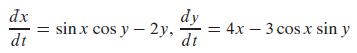
In Problems 1 through 4, show that the given system is almost linear with (0 , 0) as a critical point, and classify this critical point as to type and stability. Use a computer system or graphing calculator to construct a phase plane portrait that illustrates your conclusion. dx dt = sin x cos y -
In Problems 1 through 8, find the critical point or points of the given autonomous system, and thereby match each system with its phase portrait among Figs. 9.1.12 through 9.1.19. dx dt = 2x - 2y - 4, dy dt = x + 4y + 3
In Problems 1 through 10, apply Theorem 1 to determine the type of the critical point (0 , 0) and whether it is asymptotically stable, stable, or unstable. Verify your conclusion by using a computer system or graphing calculator to construct a phase portrait for the given linear system. dx dt = x -
Find and classify each of the critical points of the almost linear systems in Problems 5 through 8. Use a computer system or graphing calculator to construct a phase plane portrait that illustrates your findings. dx R dt = -x + sin y, dy dt = 2x
In Problems 1 through 8, find the critical point or points of the given autonomous system, and thereby match each system with its phase portrait among Figs. 9.1.12 through 9.1.19. dx dt = 1-y², dy dt = x +2y
In Problems 1 through 10, apply Theorem 1 to determine the type of the critical point (0 , 0) and whether it is asymptotically stable, stable, or unstable. Verify your conclusion by using a computer system or graphing calculator to construct a phase portrait for the given linear system. dx dt = 5x
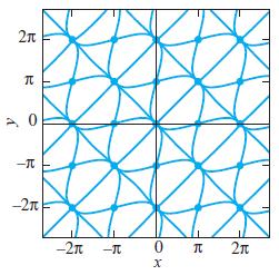
Find and classify each of the critical points of the almost linear systems in Problems 5 through 8. Use a computer system or graphing calculator to construct a phase plane portrait that illustrates your findings. dx dt = y, dy dt = sin лx - y
In Problems 1 through 8, find the critical point or points of the given autonomous system, and thereby match each system with its phase portrait among Figs. 9.1.12 through 9.1.19. dx dt = 2-4x - 15y, dy dt = 4-x²
In Problems 1 through 10, apply Theorem 1 to determine the type of the critical point (0 , 0) and whether it is asymptotically stable, stable, or unstable. Verify your conclusion by using a computer system or graphing calculator to construct a phase portrait for the given linear system.
Find and classify each of the critical points of the almost linear systems in Problems 5 through 8. Use a computer system or graphing calculator to construct a phase plane portrait that illustrates your findings. dx dt = 1- ex-y₂ dy dt 2 sin x
In Problems 1 through 8, find the critical point or points of the given autonomous system, and thereby match each system with its phase portrait among Figs. 9.1.12 through 9.1.19. dx R dt = x - 2y, dy dt = = 4x - x³
In Problems 1 through 10, apply Theorem 1 to determine the type of the critical point (0 , 0) and whether it is asymptotically stable, stable, or unstable. Verify your conclusion by using a computer system or graphing calculator to construct a phase portrait for the given linear system. dx dt = x -
Problems 8 through 10 deal with the competition systemin which c1c2 = 8 < 9 = b1b2, so the effect of inhibition should exceed that of competition. The linearization of the system in (3) at (0,0) is the same as that of (2). This observation and Problems 8 through 10 imply that the four critical
Find and classify each of the critical points of the almost linear systems in Problems 5 through 8. Use a computer system or graphing calculator to construct a phase plane portrait that illustrates your findings. dx dt 3 sin x + y, dy dt sin x + 2y
In Problems 1 through 8, find the critical point or points of the given autonomous system, and thereby match each system with its phase portrait among Figs. 9.1.12 through 9.1.19. dx dt = x - y - x² + xy, dy dt -y-x²
In Problems 1 through 10, apply Theorem 1 to determine the type of the critical point (0 , 0) and whether it is asymptotically stable, stable, or unstable. Verify your conclusion by using a computer system or graphing calculator to construct a phase portrait for the given linear system. dx dt = 2x
Problems 8 through 10 deal with the competition systemin which c1c2 = 8 < 9 = b1b2, so the effect of inhibition should exceed that of competition. The linearization of the system in (3) at (0,0) is the same as that of (2). This observation and Problems 8 through 10 imply that the four critical
In Problems 1 through 10, apply Theorem 1 to determine the type of the critical point (0, 0) and whether it is asymptotically stable, stable, or unstable. Verify your conclusion by using a computer system or graphing calculator to construct a phase portrait for the given linear system. dx dt = x -
Problems 8 through 10 deal with the competition systemin which c1c2 = 8 < 9 = b1b2, so the effect of inhibition should exceed that of competition. The linearization of the system in (3) at (0,0) is the same as that of (2). This observation and Problems 8 through 10 imply that the four critical
In Problems 9 through 12, find each equilibrium solution x(t) Ξ x0 of the given second-order differential equation x" + f(x , x') = 0. Use a computer system or graphing calculator to construct a phase portrait and direction field for the equivalent first-order system x' = y, y' = -f(x , y).
Problems 9 through 11 deal with the damped pendulum system x' = y, y' = -ω2 sinx - cy.Show that if n is an odd integer, then the critical point (nπ, 0) is a saddle point for the damped pendulum system.
Each of the systems in Problems 11 through 18 has a single critical point (x0 , y0). Apply Theorem 2 to classify this critical point as to type and stability. Verify your conclusion by using a computer system or graphing calculator to construct a phase portrait for the given system. dx dt = x -
In Problems 9 through 12, find each equilibrium solution x(t) Ξ x0 of the given second-order differential equation x" + f(x , x') = 0. Use a computer system or graphing calculator to construct a phase portrait and direction field for the equivalent first-order system x' = y, y' = -f(x, y). Thereby
Problems 9 through 11 deal with the damped pendulum system x' = y, y' = -ω2 sinx - cy.Show that if n is an even integer and c2 < 4ω2, then the critical point (nπ, 0) is a nodal sink for the damped pendulum system.
Showing 300 - 400
of 2513
1
2
3
4
5
6
7
8
9
10
11
12
13
14
15
Last
Step by Step Answers