New Semester Started Get 50% OFF Study Help! --h --m --s Claim Now

Question Answers

Textbooks

Find textbooks, questions and answers

Oops, something went wrong!

Change your search query and then try again

Result Not Found

Books FREE
Study Help
Tutors
AI Study Planner NEW
Sell Books

Search
Sign In
Register

study help
mathematics
first course differential equations

Differential Equations And Linear Algebra 4th Edition C. Edwards, David Penney, David Calvis - Solutions

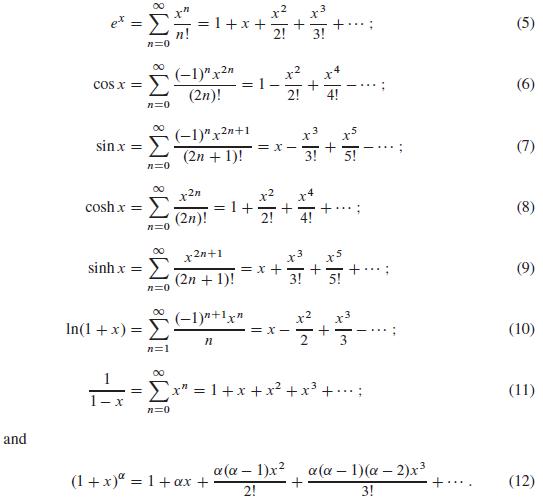
In Problems 1 through 10, find a power series solution of the given differential equation. Determine the radius of convergence of the resulting series, and use the series in Eqs. (5) through (12) to identify the series solution in terms of familiar elementary functions. and || COS X = sin.x = coshx
In Problems 1 through 8, determine whether x = 0 is an ordinary point, a regular singular point, or an irregular singular point. If it is a regular singular point, find the exponents of the differential equation at x = 0.(6x2 + 2x3)y" + 21xy' + 9(x2 - 1)y = 0
Find general solutions in powers of x of the differential equations in Problems 1 through 15. State the recurrence relation and the guaranteed radius of convergence in each case.(2 - x2)y'' - xy' + 16y = 0
In Problems 1 through 10, find a power series solution of the given differential equation. Determine the radius of convergence of the resulting series, and use the series in Eqs. (5) through (12) to identify the series solution in terms of familiar elementary functions.2 (x + 1)y' = y and || COS X
Deduce the identities in Eqs. (24) and (25) from those in Eqs. (22) and (23). dx [x² Jp(x)] = xP Jp-1(x). (22)
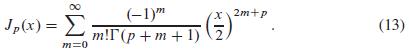
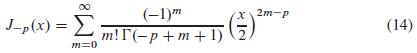
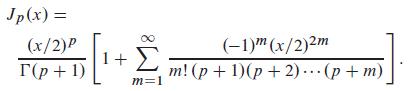
Use the relation Γ(x + 1) = xΓ(x) to deduce from Eqs. (13) and (14) that if p is not a negative integer, thenThis form is more convenient for the computation of Jp(x) because only the single value Γ (p + 1) of the gamma function is required. Jp(x) = (x/2)P T(p+1) 1 + m=1 (-1)m(x/2)2m m!
If x = a ≠ 0 is a singular point of a second-order linear differential equation, then the substitution t = x - a transforms it into a differential equation having t = 0 as a singular point. We then attribute to the original equation at x = a the behavior of the new equation at t = 0. Classify (as
Find general solutions in powers of x of the differential equations in Problems 1 through 15. State the recurrence relation and the guaranteed radius of convergence in each case.(x2 - 1)y'' + 8xy' + 12y = 0
In Problems 1 through 10, find a power series solution of the given differential equation. Determine the radius of convergence of the resulting series, and use the series in Eqs. (5) through (12) to identify the series solution in terms of familiar elementary functions.(x - 1)y' + 2y = 0 and || COS
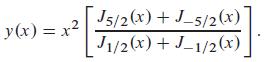
Use the series of Problem 9 to findifProblem 9Use the relation Γ(x + 1) = xΓ(x) to deduce from Eqs. (13) and (14) that if p is not a negative integer, thenThis form is more convenient for the computation of Jp(x) because only the single value Γ (p + 1) of the gamma function is required. y (0) =
If x = a ≠ 0 is a singular point of a second-order linear differential equation, then the substitution t = x - a transforms it into a differential equation having t = 0 as a singular point. We then attribute to the original equation at x = a the behavior of the new equation at t = 0. Classify (as
In Problems 1 through 10, find a power series solution of the given differential equation. Determine the radius of convergence of the resulting series, and use the series in Eqs. (5) through (12) to identify the series solution in terms of familiar elementary functions.2(x - 1)y' = 3y and || COS X
Find general solutions in powers of x of the differential equations in Problems 1 through 15. State the recurrence relation and the guaranteed radius of convergence in each case.3y'' + xy' - 4y = 0
Any integral of the form ∫ xm Jn (x) dx can be evaluated in terms of Bessel functions and the indefinite integral ∫ J0 (x) dx. The latter integral cannot be simplified further, but the function ∫x0 J0 (t) dt is tabulated in Table 11.1 of Abramowitz and Stegun. Use the identities in Eqs. (22)
In Problems 11 through 14, use the method of Example 4 to find two linearly independent power series solutions of the given differential equation. Determine the radius of convergence of each series, and identify the general solution in terms of familiar elementary functions.y'' = y Example 4 Solve
Find general solutions in powers of x of the differential equations in Problems 1 through 15. State the recurrence relation and the guaranteed radius of convergence in each case.5y'' - 2xy' + 10y = 0
If x = a ≠ 0 is a singular point of a second-order linear differential equation, then the substitution t = x - a transforms it into a differential equation having t = 0 as a singular point. We then attribute to the original equation at x = a the behavior of the new equation at t = 0. Classify (as
Any integral of the form ∫ xm Jn (x) dx can be evaluated in terms of Bessel functions and the indefinite integral ∫ J0 (x) dx. The latter integral cannot be simplified further, but the function ∫x0 J0 (t) dt is tabulated in Table 11.1 of Abramowitz and Stegun. Use the identities in Eqs. (22)
In Problems 11 through 14, use the method of Example 4 to find two linearly independent power series solutions of the given differential equation. Determine the radius of convergence of each series, and identify the general solution in terms of familiar elementary functions.y'' = 4y Example 4 Solve
Find general solutions in powers of x of the differential equations in Problems 1 through 15. State the recurrence relation and the guaranteed radius of convergence in each case.y'' - x2y' - 3xy = 0
If x = a ≠ 0 is a singular point of a second-order linear differential equation, then the substitution t = x - a transforms it into a differential equation having t = 0 as a singular point. We then attribute to the original equation at x = a the behavior of the new equation at t = 0. Classify (as
Any integral of the form ∫ xm Jn (x) dx can be evaluated in terms of Bessel functions and the indefinite integral ∫ J0 (x) dx. The latter integral cannot be simplified further, but the function ∫x0 J0 (t) dt is tabulated in Table 11.1 of Abramowitz and Stegun. Use the identities in Eqs. (22)
In Problems 11 through 14, use the method of Example 4 to find two linearly independent power series solutions of the given differential equation. Determine the radius of convergence of each series, and identify the general solution in terms of familiar elementary functions.y'' + 9y = 0 Example
Find general solutions in powers of x of the differential equations in Problems 1 through 15. State the recurrence relation and the guaranteed radius of convergence in each case.y'' + x2y' + 2xy = 0
In Problems 1 through 8, apply the successive approximation formula to compute yn (x) for n ≦ 4. Then write the exponential series for which these approximations are partial sums (perhaps with the first term or two missing; for example, e* - 1 = x + x² + x³ + 1/ 4x -214x² + ...).
In Problems 1 through 8, apply the successive approximation formula to compute yn (x) for n ≦ 4. Then write the exponential series for which these approximations are partial sums (perhaps with the first term or two missing; for example, e* - 1 = x + x² + x³ + 1/ 4x -214x² + ...).
In Problems 1 through 8, apply the successive approximation formula to compute yn (x) for n ≦ 4. Then write the exponential series for which these approximations are partial sums (perhaps with the first term or two missing; for example, e* - 1 = x + x² + x³ + 1/ 4x -214x² + ...).
In Problems 1 through 8, apply the successive approximation formula to compute yn (x) for n ≦ 4. Then write the exponential series for which these approximations are partial sums (perhaps with the first term or two missing; for example, e* - 1 = x + x² + x³ + 1/ 4x -214x² + ...).
In Problems 1 through 8, apply the successive approximation formula to compute yn (x) for n ≦ 4. Then write the exponential series for which these approximations are partial sums (perhaps with the first term or two missing; for example, e* - 1 = x + x² + x³ + 1/ 4x -214x² + ...).
In Problems 1 through 8, apply the successive approximation formula to compute yn (x) for n ≦ 4. Then write the exponential series for which these approximations are partial sums (perhaps with the first term or two missing; for example, e* - 1 = x + x² + x³ + 1/ 4x -214x² + ...).
In Problems 1 through 8, apply the successive approximation formula to compute yn (x) for n ≦ 4. Then write the exponential series for which these approximations are partial sums (perhaps with the first term or two missing; for example, e* - 1 = x + x² + x³ + 1/ 4x -214x² + ...).
In Problems 1 through 8, apply the successive approximation formula to compute yn (x) for n ≦ 4. Then write the exponential series for which these approximations are partial sums (perhaps with the first term or two missing; for example, e* - 1 = x + x² + x³ + 1/ 4x -214x² + ...).
In Problems 9 through 12, compute the successive approximations yn (x) for n ≦ 3; then compare them with the appropriate partial sums of the Taylor series of the exact solution. dy dx = x + y, y(0) = 1
In Problems 9 through 12, compute the successive approximations yn (x) for n ≦ 3; then compare them with the appropriate partial sums of the Taylor series of the exact solution. dy dx = y + e*, y(0) = 0
In Problems 9 through 12, compute the successive approximations yn (x) for n ≦ 3; then compare them with the appropriate partial sums of the Taylor series of the exact solution. dy dx = y2, y(0) = 1
In Problems 9 through 12, compute the successive approximations yn (x) for n ≦ 3; then compare them with the appropriate partial sums of the Taylor series of the exact solution. dy dx = y³, y(0) = 1
Apply the iterative formula in (16) to compute the first three successive approximations to the solution of the initial value problem dx dt dy dt = 2x - y, = 3x - 2y, x(0) = 1; y(0) = -1.
Apply the matrix exponential in (19) to solve (in closed form) the initial value problemShow first thatfor each positive integer n.) [i]=0x X, x(0) [B].
A programmable calculator or a computer will be useful for Problems 11 through 16. In each problem find the exact solution of the given initial value problem. Then apply Euler’s method twice to approximate (to four decimal places) this solution on the given interval, first with step size h =
A programmable calculator or a computer will be useful for Problems 11 through 16. In each problem find the exact solution of the given initial value problem. Then apply Euler’s method twice to approximate (to four decimal places) this solution on the given interval, first with step size h =
A programmable calculator or a computer will be useful for Problems 11 through 16. In each problem find the exact solution of the given initial value problem. Then apply Euler’s method twice to approximate (to four decimal places) this solution on the given interval, first with step size h =
A programmable calculator or a computer will be useful for Problems 11 through 16. In each problem find the exact solution of the given initial value problem. Then apply Euler’s method twice to approximate (to four decimal places) this solution on the given interval, first with step size h =
A programmable calculator or a computer will be useful for Problems 11 through 16. In each problem find the exact solution of the given initial value problem. Then apply Euler’s method twice to approximate (to four decimal places) this solution on the given interval, first with step size h =
A programmable calculator or a computer will be useful for Problems 11 through 16. In each problem find the exact solution of the given initial value problem. Then apply Euler’s method twice to approximate (to four decimal places) this solution on the given interval, first with step size h =
A hand-held calculator will suffice for Problems 1 through 10, where an initial value problem and its exact solution are given. Apply the improved Euler method to approximate this solution on the interval [0, 0.5] with step size h = 0.1. Construct a table showing four-decimal-place values of the
Separate variables and use partial fractions to solve the initial value problems in Problems 1–8. Use either the exact solution or a computer-generated slope field to sketch the graphs of several solutions of the given differential equation, and highlight the indicated particular solution.
A hand-held calculator will suffice for Problems 1 through 10, where an initial value problem and its exact solution are given. Apply the improved Euler method to approximate this solution on the interval [0, 0.5] with step size h = 0.1. Construct a table showing four-decimal-place values of the
A hand-held calculator will suffice for Problems 1 through 10, where an initial value problem and its exact solution are given. Apply the Runge–Kutta method to approximate this solution on the interval [0,0.5]? with step size h = 0.25. Construct a table showing five-decimal-place values of the
A hand-held calculator will suffice for Problems 1 through 10, where an initial value problem and its exact solution are given. Apply the improved Euler method to approximate this solution on the interval [0, 0.5] with step size h = 0.1. Construct a table showing four-decimal-place values of the
A hand-held calculator will suffice for Problems 1 through 10, where an initial value problem and its exact solution are given. Apply the improved Euler method to approximate this solution on the interval [0, 0.5] with step size h = 0.1. Construct a table showing four-decimal-place values of the
A computer with a printer is required for Problems 17 through 24. In these initial value problems, use Euler’s method with step sizes h = 0.1, 0.02, 0.004, and 0.0008 to approximate to four decimal places the values of the solution at ten equally spaced points of the given interval. Print the
A computer with a printer is required for Problems 17 through 24. In these initial value problems, use the Runge–Kutta method with step sizes h = 0.2, 0.1, 0.05, and 0.025 to approximate to six decimal places the values of the solution at five equally spaced points of the given interval. Print
A hand-held calculator will suffice for Problems 1 through 10, where an initial value problem and its exact solution are given. Apply the Runge–Kutta method to approximate this solution on the interval [0,0.5] with step size h = 0.25. Construct a table showing five-decimal-place values of the
A hand-held calculator will suffice for Problems 1 through 10, where an initial value problem and its exact solution are given. Apply the Runge–Kutta method to approximate this solution on the interval [0,0.5]? with step size h = 0.25. Construct a table showing five-decimal-place values of the
A hand-held calculator will suffice for Problems 1 through 10, where an initial value problem and its exact solution are given. Apply the improved Euler method to approximate this solution on the interval [0, 0.5] with step size h = 0.1. Construct a table showing four-decimal-place values of the
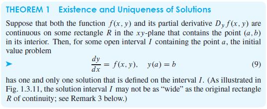
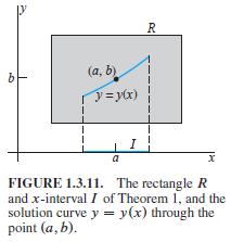
A more detailed version of Theorem 1 says that, if the function f (x, y) is continuous near the point (a, b), then at least one solution of the differential equation y' = f (x, y) exists on some open interval I containing the point x = a and, moreover, that if in addition the partial derivative
Each of Problems 43 through 48 gives a general solution y(x) of a homogeneous second-order differential equation ay'' + by' + cy = 0 with constant coefficients. Find such an equation.y(x) = c1e10x + c2e100x
Each of Problems 43 through 48 gives a general solution y(x) of a homogeneous second-order differential equation ay'' + by' + cy = 0 with constant coefficients. Find such an equation. y(x) = ex (c₁ex√² + + c₂e-x√√2)
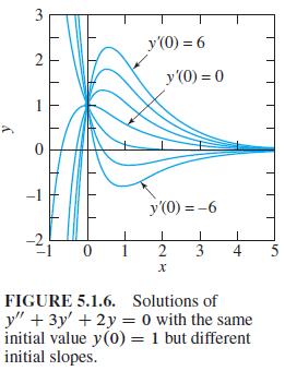
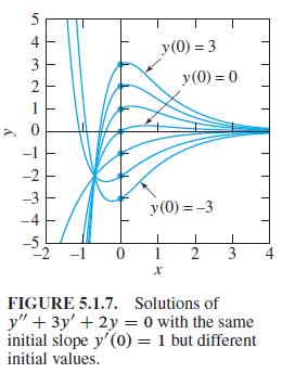
Problems 49 and 50 deal with the solution curves of y'' + 3y' + 2y = 0 shown in Figs. 5.1.6 and 5.1.7.Figure 5.1.7 suggests that the solution curves shown all meet at a common point in the third quadrant. Assuming that this is indeed the case, find the coordinates of that point. 3 2 T 0 - y'(0) =
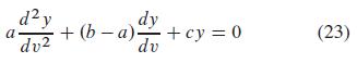
A second-order Euler equation is one of the formwhere a, b, c are constants.(a) Show that if x > 0, then the substitution v = ln x transforms Eq. (22) into the constant- coefficient linear equationwith independent variable v.(b) If the roots r1 and r2 of the characteristic equation of Eq. (23)
Make the substitution v = ln x of Problem 51 to find general solutions (for x > 0) of the Euler equations in Problems 52–56.x2y'' + xy' - y = 0
Make the substitution v = ln x of Problem 51 to find general solutions (for x > 0) of the Euler equations in Problems 52–56.x2y'' + 2xy' - 12y = 0
Make the substitution v = ln x of Problem 51 to find general solutions (for x > 0) of the Euler equations in Problems 52–56.4x2y'' + 8xy' - 3y = 0
Make the substitution v = ln x of Problem 51 to find general solutions (for x > 0) of the Euler equations in Problems 52–56.x2y'' - 3xy' + 4y = 0
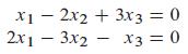
In Problems 15–26, find a basis for the solution space of the given homogeneous linear system. x12x2 + 3x3 = 2x13x2x3 = 0
In Problems 13–18, determine whether the given functions are linearly independent.1 + x, 1 - x, and 1 - x2
In Problems 17–22, three vectors v1, v2, and v3 are given. If they are linearly independent, show this; otherwise find a nontrivial linear combination of them that is equal to the zero vector.v1 = (2,0, -3), v2 = (4, -5, -6), v3 = (-2,1,3)
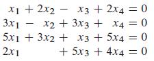
In Problems 15–26, find a basis for the solution space of the given homogeneous linear system. x1 + 3x2 + 4x3 + 5x4 = 0 2x1 + 6x2 + 9x3 + 5x4 = 0
In Problems 13–22, the given vectors span a subspace V of the indicated Euclidean space. Find a basis for the orthogonal complement V⊥ of V.v1 = (1, -3, 3, 5), v2 = (2,-5, 9, 3)
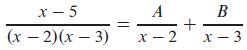
In Problems 19–22, use the method of Example 5 to find the constants A, B, and C in the indicated partial-fraction decompositions. x-5 (x-2)(x-3) A x-2 + B x 3
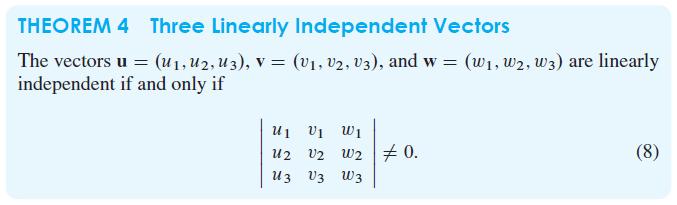
In Problems 15–18, apply Theorem 4 (that is, calculate a determinant) to determine whether the given vectors u, v, and w are linearly dependent or independent.u = (1, 1, 0), v = (4, 3, 1), w = (3, -2, -4) THEOREM 4 Three Linearly Independent Vectors The vectors u = (₁, U2, U3), V = (v₁, V2,
In Problems 13–18, determine whether the given functions are linearly independent.2 cos x + 3 sin x and 4 cos x + 5 sin x
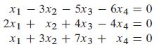
In Problems 19–22, reduce the given system to echelon form to find a single solution vector u such that the solution space is the set of all scalar multiples of u. x13x25x3 - 6x4 = 0 2x1 + x2 + 4x3 4x4 = 0 x1 + 3x2 + 7x3 + x4 = 0
In Problems 17–22, three vectors v1, v2, and v3 are given. If they are linearly independent, show this; otherwise find a nontrivial linear combination of them that is equal to the zero vector.v1 = (2,0,3,0), v2 = (5, 4, -2, 1), v3 = (2,-1,1,-1)
In Problems 13–22, the given vectors span a subspace V of the indicated Euclidean space. Find a basis for the orthogonal complement V⊥ of V.v1 = (1, 2, 5, 2, 3), v2 = (3, 7, 11, 9,5)
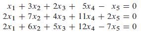
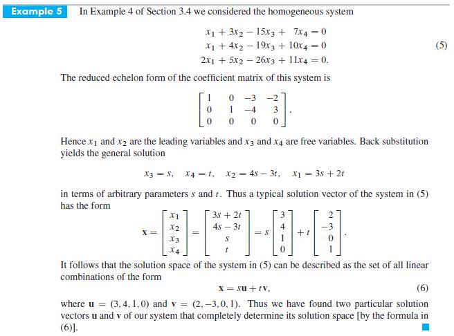
In Problems 15–18, apply the method of Example 5 to find two solution vectors u and v such that the solution space is the set of all linear combinations of the form su + tv. X5 = 0 x1 + 3x2 + 2x3 + 5x4- 2x1 + 7x2 + 4x3 + 11x4 + 2x5 = 0 2x1 + 6x2 + 5x3 + 12x47x5 = 0
Let S = {v1, v2, ...., vk} be a basis for the subspace W of Rn. Then a basis T for Rn that contains S can be found by applying the method of Example 5 to the vectorsv1, v2, ......, vk, e1, e2, ......, en.Do this in Problems 17–20.Find a basis T for R3 that contains the vectors v1 = (3,2,-1) and
Let S = {v1, v2, ...., vk} be a basis for the subspace W of Rn. Then a basis T for Rn that contains S can be found by applying the method of Example 5 to the vectorsv1, v2, ......, vk, e1, e2, ......, en.Do this in Problems 17–20.Find a basis T for R3 that contains the vectors v1 = (1, 2, 2) and
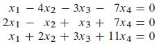
In Problems 15–18, apply the method of Example 5 to find two solution vectors u and v such that the solution space is the set of all linear combinations of the form su + tv. x14x2 3x3 - - 7x4 = 0 2x1 - x₂ + x3 + 7x4 = 0 x2 x1 + 2x2 + 3x3 + 11x4 = 0
In Problems 9–16, express the indicated vector w as a linear combination of the given vectors v1, v2, ....., vk if this is possible. If not, show that it is impossible.w = (7,7,9, 11); v1 = (2,0, 3, 1), v2 = (4, 1, 3, 2), v3 = (1,3,-1,3)
In Problems 13–22, the given vectors span a subspace V of the indicated Euclidean space. Find a basis for the orthogonal complement V⊥ of V.v1 = (1, 7, -6, -9)
In Problems 13–16, a set S of vectors in R4 is given. Find a subset of S that forms a basis for the subspace of R4 spanned by S.v1 = (5,4,2,2), v2 = (3,1,2,3), v3 = (7,7,2,1), v4 = (1,-1,2,4), v5 = (5,4,6,7)
In Problems 13–18, determine whether the given functions are linearly independent.cos 2x, sin2 x, and cos2 x
In Problems 15–18, apply Theorem 4 (that is, calculate a determinant) to determine whether the given vectors u, v, and w are linearly dependent or independent.u = (1, -1, 2), v = (3, 0, 1), w = (1, -2, 2) THEOREM 4 Three Linearly Independent Vectors The vectors u = (₁, U2, U3), V = (v₁, V2,
In Problems 15–26, find a basis for the solution space of the given homogeneous linear system. x13x2 2x15x2 + 2x3 - 4x4 = 0 + 7x3 3x4 = 0
In Problems 15–26, find a basis for the solution space of the given homogeneous linear system. x1 + 3x2 + 4x3 = 0 3x1 + 8x2 + 7x3 =
In Problems 13–22, the given vectors span a subspace V of the indicated Euclidean space. Find a basis for the orthogonal complement V⊥ of V.v1 = (1, 3, 2, 4), v2 = (2,7,7,3)
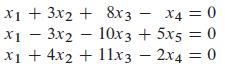
In Problems 15–18, apply the method of Example 5 to find two solution vectors u and v such that the solution space is the set of all linear combinations of the form su + tv. x1 + 3x2 + 8x3 x4 = 0 x13x210x3 + 5x5 = 0 x1 + 4x2 + 11x3 - 2x4 = 0
In Problems 17–22, three vectors v1, v2, and v3 are given. If they are linearly independent, show this; otherwise find a nontrivial linear combination of them that is equal to the zero vector.v1 = (1, 0, 1), v2 = (2,-3, 4), v3 = (3,5,2)
In Problems 15–18, apply Theorem 4 (that is, calculate a determinant) to determine whether the given vectors u, v, and w are linearly dependent or independent.u = (5, -2, 4), v = (2, -3, 5), w = (4, 5, -7) THEOREM 4 Three Linearly Independent Vectors The vectors u = (₁, U2, U3), V = (v₁, V2,
In Problems 13–18, determine whether the given functions are linearly independent.1 + x, x + x2, and 1 - x2
In Problems 23 and 24, use the method of Example 7 to find a basis for the solution space of the given differential equation. (It’s 3-dimensional in Problem 23 and 4-dimensional in Problem 24.)y''' = 0 Example 7 With a = 1 and b = c = 0 in (16), we get the differential equation y" = 0. (17)
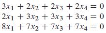
Given a homogeneous system Ax = 0 of (scalar) linear equations, we say that a subset of these equations is irredundant provided that the corresponding column vectors of the transpose AT are linearly independent. In Problems 21–24, extract from each given system a maximal subset of
In Problems 23–26, the vectors {vi} are known to be linearly independent. Apply the definition of linear independence to show that the vectors {ui} are also linearly independent.u1 = v1 + v2, u2 = v1 - v2
In Problems 19–24, use the method of Example 3 to determine whether the given vectors u, v, and w are linearly independent or dependent. If they are linearly dependent, find scalars a, b, and c not all zero such that au + bv + cw = 0.u = (2,0, 3), v = (5,4,-2), w = (2,-1,1)
Prove: For arbitrary vectors u and v,(a) |u + v|2 + |u - v|2 = 2|u|2 + 2|v|2;(b) |u + v|2 - |u - v|2 = 4u . v.
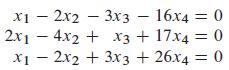
In Problems 15–26, find a basis for the solution space of the given homogeneous linear system. x12x2 3x3 - 16x4 – 2x14x2 x12x2 16x4 = 0 + x3 + 17x4 = 0 + 3x3 +26x4: = 0
In Problems 13–22, the given vectors span a subspace V of the indicated Euclidean space. Find a basis for the orthogonal complement V⊥ of V.v1 = (1, 1, 1, 1, 3), v2 = (2, 3, 1, 4, 7), v3 = (5,3,7,1,5)
In Problems 17–22, three vectors v1, v2, and v3 are given. If they are linearly independent, show this; otherwise find a nontrivial linear combination of them that is equal to the zero vector.v1 = (3,9, 0,5), v2 = (3, 0, 9,-7), v3 = (4,7,5,0)
Given a homogeneous system Ax = 0 of (scalar) linear equations, we say that a subset of these equations is irredundant provided that the corresponding column vectors of the transpose AT are linearly independent. In Problems 21–24, extract from each given system a maximal subset of

Showing 1300 - 1400 of 2513

First
7
8
9
10
11
12
13
14
15
16
17
18
19
20
21
Last

Step by Step Answers

Services

Sitemap
Fun
Definitions
Become Tutor
Used Textbooks
Study Help Categories
Recent Questions
Expert Questions
Campus Wear
Sell Your Books

Company Info

Security
Copyrights
Privacy Policy
Terms & Conditions
SolutionInn Fee
Scholarship
Online Quiz
Give Feedback, Get Rewards

Get In Touch

About Us
Contact Us
Career
Jobs
FAQ
Student Discount
Campus Ambassador

Secure Payment

Download Our App

© 2026 SolutionInn. All Rights Reserved