New Semester Started Get 50% OFF Study Help! --h --m --s Claim Now

Question Answers

Textbooks

Find textbooks, questions and answers

Oops, something went wrong!

Change your search query and then try again

Result Not Found

Books FREE
Study Help
Tutors
AI Study Planner NEW
Sell Books

Search
Sign In
Register

study help
mathematics
first course differential equations

Differential Equations And Linear Algebra 4th Edition C. Edwards, David Penney, David Calvis - Solutions

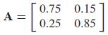
In Problems 25 through 30, a city-suburban population transition matrix A (as in Example 2) is given. Find the resulting long-term distribution of a constant total population between the city and its suburbs. A = 0.75 0.15 0.25 0.85
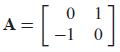
Find the complex conjugate eigenvalues and corresponding eigenvectors of the matrices given in Problems 27 through 32. 01 A = [_- ] -1 0
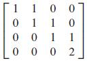
In Problems 1 through 28, determine whether or not the given matrix A is diagonalizable. If it is, find a diagonalizing matrix P and a diagonal matrix D such that P-1 AP = D. 1 1 0 0 01 10 0 0 1 1 0002
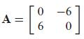
Find the complex conjugate eigenvalues and corresponding eigenvectors of the matrices given in Problems 27 through 32. =[% A = -6 0
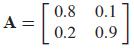
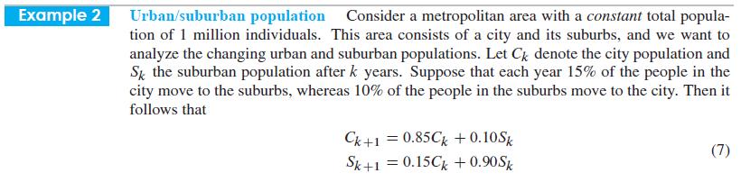
In Problems 25 through 30, a city-suburban population transition matrix A (as in Example 2) is given. Find the resulting long-term distribution of a constant total population between the city and its suburbs. =[8 Α = 0.8 0.2 0.1 0.9
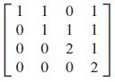
In Problems 1 through 28, determine whether or not the given matrix A is diagonalizable. If it is, find a diagonalizing matrix P and a diagonal matrix D such that P-1 AP = D. 1 1 0 0 1 1 1 1 0021 0002
Find the complex conjugate eigenvalues and corresponding eigenvectors of the matrices given in Problems 27 through 32. A = 0 12 -3 0
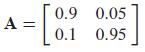
In Problems 25 through 30, a city-suburban population transition matrix A (as in Example 2) is given. Find the resulting long-term distribution of a constant total population between the city and its suburbs. 0.9 0.05 0.1 0.95 Α A = [0.1
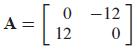
Find the complex conjugate eigenvalues and corresponding eigenvectors of the matrices given in Problems 27 through 32. A = 0-12 0 12
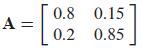
In Problems 25 through 30, a city-suburban population transition matrix A (as in Example 2) is given. Find the resulting long-term distribution of a constant total population between the city and its suburbs. A = [8 0.8 0.15 0.2 0.85
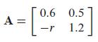
Problems 31 through 33 deal with a fox-rabbit population as in Examples 3 through 5, except with the transition matrixin place of the one used in the text.If r = 0.16, show that in the long term the populations of foxes and rabbits are stable, with 5 foxes for each 4 rabbits. = [06 A 0.6 0.5 1.2
Find the complex conjugate eigenvalues and corresponding eigenvectors of the matrices given in Problems 27 through 32. ·[₁ A = 0 -6 24 0
Problems 31 through 33 deal with a fox-rabbit population as in Examples 3 through 5, except with the transition matrixin place of the one used in the text.If r = 0.175, show that in the long term the populations of foxes and rabbits both die out. = [06 A 0.6 0.5 1.2
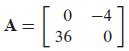
Find the complex conjugate eigenvalues and corresponding eigenvectors of the matrices given in Problems 27 through 32. = [3% 36 A = 0-4 0 ]
Problems 31 through 33 deal with a fox-rabbit population as in Examples 3 through 5, except with the transition matrixin place of the one used in the text.If r = 0.135, show that in the long term the fox and rabbit populations both increase at the rate of 5% per month, maintaining a constant ratio
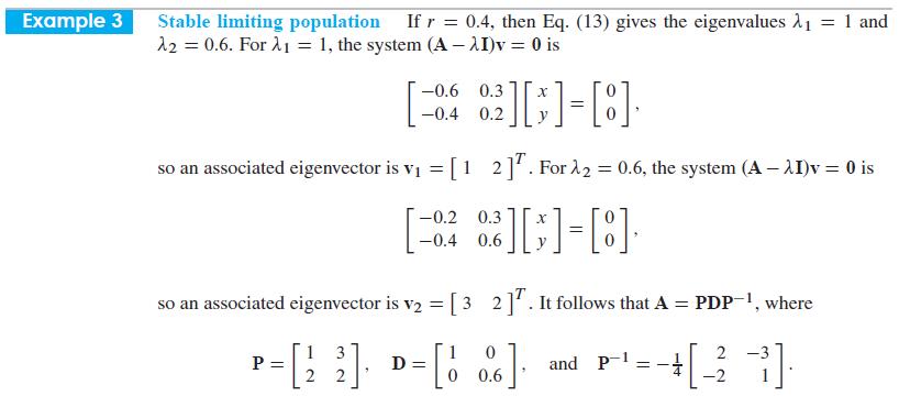
Suppose that the 2 x 2 matrix A has eigenvalues λ1 = 1 and λ2 = -1 with eigenvectors v1 = (3, 4) and v2 = (5,7), respectively. Find the matrix A and the powers A99 and A100.
Suppose thatShow that A2n = I and that A2n+1 = A for every positive integer n. 01 =[i]. 1 0 A =
Let A be a 3 x 3 matrix with three distinct eigenvalues. Tell how to construct six different invertible matrices P1, P2,..., P6 and six different diagonal matrices D1, D2,..., D6 such that PiDi (Pi)-1 = A for each i = 1,2,..., 6.
Suppose that the characteristic equation |A - λI| = 0 is written as a polynomial equation [Eq. (5)]. Show that the constant term is c0 = det A. (-1)^2n + Cn-12²¹ +...+c₁d + co = 0, (5)
Suppose thatShow that A4n = I, A4n+1 = A, A4n+2 = -I, and A4n+3 = -A for every positive integer n. A=[- 0 8]. 0
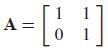
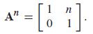
The matrixis not diagonalizable. (Why not?) Write A = I + B. Show that B2 = 0 and thence that A = [1₂] 0
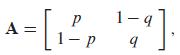
Consider the stochastic matrixwhere 0 < p < 1 and 0 < q < 1. Show that the eigenvalues of A are λ1 = 1 and λ2 = p + q - 1, so that |λ2| < 1. P 1-q A = [1²₂ ¹-9]. 1-
In Problems 1 through 16, apply the eigenvalue method of this section to find a general solution of the given system. If initial values are given, find also the corresponding particular solution. For each problem, use a computer system or graphing calculator to construct a direction field and
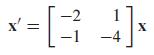
Find general solutions of the systems in Problems 1 through 22. In Problems 1 through 6, use a computer system or graphing calculator to construct a direction field and typical solution curves for the given system. X X I- [□]=x I
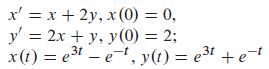
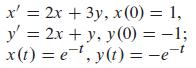
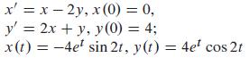
A hand-held calculator will suffice for Problems 1 through 8. In each problem an initial value problem and its exact solution are given. Approximate the values of x (0.2) and y(0.2) in three ways:(a) By the Euler method with two steps of size h = 0.1;(b) by the improved Euler method with a single
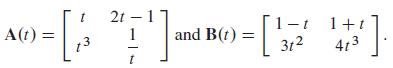
In Problems 1 and 2, verify the product law for differentiation, (AB)' = A'B + AB'. A(t) = t 3 1 2t - 1 2¹] and B() = ['172² t 1+t 413 1.
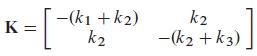
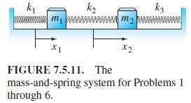
Problems 1 through 7 deal with the mass-and-spring system shown in Fig. 7.5.11 with stiffness matrixand with the given mks values for the masses and spring constants. Find the two natural frequencies of the system and describe its two natural modes of oscillation.m1 = m2 = 1; k1 = 1, k2 = 4, k3 = 1
In Problems 1 through 16, apply the eigenvalue method of this section to find a general solution of the given system. If initial values are given, find also the corresponding particular solution. For each problem, use a computer system or graphing calculator to construct a direction field and
In Problems 1 through 10, transform the given differential equation or system into an equivalent system of first-order differential equations.x'' + 3x' + 7x = t2
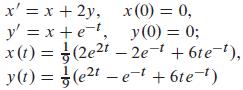
A hand-held calculator will suffice for Problems 1 through 8. In each problem an initial value problem and its exact solution are given. Approximate the values of x (0.2) and y(0.2) in three ways:(a) By the Euler method with two steps of size h = 0.1;(b) By the improved Euler method with a
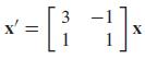
Find general solutions of the systems in Problems 1 through 22. In Problems 1 through 6, use a computer system or graphing calculator to construct a direction field and typical solution curves for the given system. = [11] 3 -1 X' X
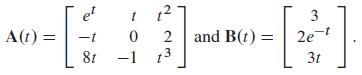
In Problems 1 and 2, verify the product law for differentiation, (AB)' = A'B + AB'. et -[₁ -t 8t A (t) = t 0 -1 1² 2 and B(t) = 13 3 2e-t 3t
In Problems 1 through 16, apply the eigenvalue method of this section to find a general solution of the given system. If initial values are given, find also the corresponding particular solution. For each problem, use a computer system or graphing calculator to construct a direction field and
In Problems 1 through 10, transform the given differential equation or system into an equivalent system of first-order differential equations.x(4) + 6x" - 3x' + x = cos 3t
In Problems 3 through 12, write the given system in the form x' = P(t)x + f(t).x' = tx - et y + cost, y' = e-t x + t2y - sint
Problems 1 through 7 deal with the mass-and-spring system shown in Fig. 7.5.11 with stiffness matrixand with the given mks values for the masses and spring constants. Find the two natural frequencies of the system and describe its two natural modes of oscillation.m1 = m2 = 1; k1 = 0, k2 = 2, k3 = 0
Suppose that A is an n x n stochastic matrix—the sum of the elements of each column vector is 1. If v = (1, 1, .... 1), show that AT v = v. Why does it follow that λ = 1 is an eigenvalue of A?
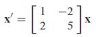
Find general solutions of the systems in Problems 1 through 22. In Problems 1 through 6, use a computer system or graphing calculator to construct a direction field and typical solution curves for the given system. X 1 -2 = [₁2 X 5
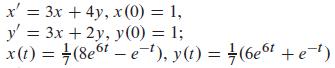
A hand-held calculator will suffice for Problems 1 through 8. In each problem an initial value problem and its exact solution are given. Approximate the values of x (0.2) and y(0.2) in three ways:(a) By the Euler method with two steps of size h = 0.1;(b) by the improved Euler method with a single
Problems 1 through 7 deal with the mass-and-spring system shown in Fig. 7.5.11 with stiffness matrixand with the given mks values for the masses and spring constants. Find the two natural frequencies of the system and describe its two natural modes of oscillation.m1 = m2 = 1; k1 = 1, k2 = 2, k3 = 1
In Problems 3 through 12, write the given system in the form x' = P(t)x + f(t).x' = -3y, y' = 3x
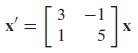
Find general solutions of the systems in Problems 1 through 22. In Problems 1 through 6, use a computer system or graphing calculator to construct a direction field and typical solution curves for the given system. x = [₁ 1 3-1 5 X
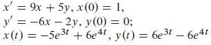
A hand-held calculator will suffice for Problems 1 through 8. In each problem an initial value problem and its exact solution are given. Approximate the values of x (0.2) and y(0.2) in three ways:(a) By the Euler method with two steps of size h = 0.1;(b) By the improved Euler method with a single
In Problems 1 through 16, apply the eigenvalue method of this section to find a general solution of the given system. If initial values are given, find also the corresponding particular solution. For each problem, use a computer system or graphing calculator to construct a direction field and
In Problems 1 through 10, transform the given differential equation or system into an equivalent system of first-order differential equations.t2 x" + tx' + (t2 - 1)x = 0
Problems 1 through 7 deal with the mass-and-spring system shown in Fig. 7.5.11 with stiffness matrixand with the given mks values for the masses and spring constants. Find the two natural frequencies of the system and describe its two natural modes of oscillation.m1 = m2 = 1; k1 = 2, k2 = 1, k3 = 2
In Problems 3 through 12, write the given system in the form x' = P(t)x + f(t).x' = 3x - 2y, y' = 2x + y
In Problems 1 through 16, apply the eigenvalue method of this section to find a general solution of the given system. If initial values are given, find also the corresponding particular solution. For each problem, use a computer system or graphing calculator to construct a direction field and
In Problems 1 through 10, transform the given differential equation or system into an equivalent system of first-order differential equations.t3 x(3) - 2t2x" + 3tx' + 5x = Int
A hand-held calculator will suffice for Problems 1 through 8. In each problem an initial value problem and its exact solution are given. Approximate the values of x (0.2) and y(0.2) in three ways:(a) By the Euler method with two steps of size h = 0.1;(b) by the improved Euler method with a single
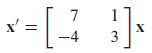
Find general solutions of the systems in Problems 1 through 22. In Problems 1 through 6, use a computer system or graphing calculator to construct a direction field and typical solution curves for the given system. 7 -4 -[- 13] x X
In Problems 3 through 12, write the given system in the form x' = P(t)x + f(t).x' = 2x + 4y + 3et, y' = 5x - y - t2
Problems 1 through 7 deal with the mass-and-spring system shown in Fig. 7.5.11 with stiffness matrixand with the given mks values for the masses and spring constants. Find the two natural frequencies of the system and describe its two natural modes of oscillation.m1 = 1 , m2 = 2; k1 = 2, k2 = k3 =
In Problems 1 through 10, transform the given differential equation or system into an equivalent system of first-order differential equations.x(3) = (x')2 + cos x
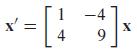
Find general solutions of the systems in Problems 1 through 22. In Problems 1 through 6, use a computer system or graphing calculator to construct a direction field and typical solution curves for the given system. 1 = [4 -4 9 X
In Problems 1 through 16, apply the eigenvalue method of this section to find a general solution of the given system. If initial values are given, find also the corresponding particular solution. For each problem, use a computer system or graphing calculator to construct a direction field and
A hand-held calculator will suffice for Problems 1 through 8. In each problem an initial value problem and its exact solution are given. Approximate the values of x (0.2) and y(0.2) in three ways:(a) By the Euler method with two steps of size h = 0.1;(b) by the improved Euler method with a single
Problems 1 through 7 deal with the mass-and-spring system shown in Fig. 7.5.11 with stiffness matrixand with the given mks values for the masses and spring constants. Find the two natural frequencies of the system and describe its two natural modes of oscillation.m1 = m2 = 1; k1 = 4, k2 = 6, k3 = 4
In Problems 1 through 16, apply the eigenvalue method of this section to find a general solution of the given system. If initial values are given, find also the corresponding particular solution. For each problem, use a computer system or graphing calculator to construct a direction field and
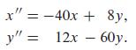
In Problems 1 through 10, transform the given differential equation or system into an equivalent system of first-order differential equations.x" - 5x + 4y = 0, y" + 4x - 5y = 0
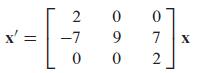
Find general solutions of the systems in Problems 1 through 22. In Problems 1 through 6, use a computer system or graphing calculator to construct a direction field and typical solution curves for the given system. x' = 2 -7 0 0 9 0 0 7 2 X
A hand-held calculator will suffice for Problems 1 through 8. In each problem an initial value problem and its exact solution are given. Approximate the values of x (0.2) and y(0.2) in three ways:(a) By the Euler method with two steps of size h = 0.1;(b) by the improved Euler method with a single
In Problems 1 through 10, transform the given differential equation or system into an equivalent system of first-order differential equations. = kx (x² + y2)3/2¹ 2 , y" ky (x2 + y2)3/2
In Problems 3 through 12, write the given system in the form x' = P(t)x + f(t).x' = y + z, y' = z + x z' = x + y
In Problems 1 through 16, apply the eigenvalue method of this section to find a general solution of the given system. If initial values are given, find also the corresponding particular solution. For each problem, use a computer system or graphing calculator to construct a direction field and
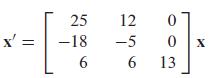
Find general solutions of the systems in Problems 1 through 22. In Problems 1 through 6, use a computer system or graphing calculator to construct a direction field and typical solution curves for the given system. X' x = 25 -18 6 12 -5 56 6 0 0 13 X
In Problems 1 through 16, apply the eigenvalue method of this section to find a general solution of the given system. If initial values are given, find also the corresponding particular solution. For each problem, use a computer system or graphing calculator to construct a direction field and
In Problems 8 through 10 the indicated mass-and-spring system is set in motion from rest (x'1 (0) = x'2 (0) = 0) in its equilibrium position (x1(0) = x2(0) = 0) with the given external forces F1(t) and F2(t) acting on the masses m1 and m2, respectively. Find the resulting motion of the system and
In Problems 3 through 12, write the given system in the form x' = P(t)x + f(t).x' = 2x - 3y, y' = x + y + 2z, z' = 5y - 7z
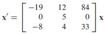
Find general solutions of the systems in Problems 1 through 22. In Problems 1 through 6, use a computer system or graphing calculator to construct a direction field and typical solution curves for the given system. x' = L -19 0 -8 12 5 4 84 0 33 X
In Problems 1 through 10, transform the given differential equation or system into an equivalent system of first-order differential equations.x" + 3x' + 4x - 2y = 0, y" + 2y' - 3x + y = cost
A computer will be required for the remaining problems in this section. In Problems 9 through 12, an initial value problem and its exact solution are given. In each of these four problems, use the Runge–Kutta method with step sizes h = 0.1 and h = 0.05 to approximate to five decimal places the
In Problems 8 through 10 the indicated mass-and-spring system is set in motion from rest (x'1 (0) = x'2 (0) = 0) in its equilibrium position (x1(0) = x2(0) = 0) with the given external forces F1(t) and F2(t) acting on the masses m1 and m2, respectively. Find the resulting motion of the system and
In Problems 1 through 16, apply the eigenvalue method of this section to find a general solution of the given system. If initial values are given, find also the corresponding particular solution. For each problem, use a computer system or graphing calculator to construct a direction field and
In Problems 3 through 12, write the given system in the form x' = P(t)x + f(t).x' = 3x - 4y + z + t, y' = x - 3z + t2, z' = 6y - 7z + t3
In Problems 1 through 10, transform the given differential equation or system into an equivalent system of first-order differential equations.x" = 3x - y + 2z, y" = x + y - 4z, z" = 5x - y - z
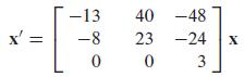
Find general solutions of the systems in Problems 1 through 22. In Problems 1 through 6, use a computer system or graphing calculator to construct a direction field and typical solution curves for the given system. x = -13 40 -48 -8 23 -24 0 0 3 X
A computer will be required for the remaining problems in this section. In Problems 9 through 12, an initial value problem and its exact solution are given. In each of these four problems, use the Runge–Kutta method with step sizes h = 0.1 and h = 0.05 to approximate to five decimal places the
In Problems 8 through 10 the indicated mass-and-spring system is set in motion from rest (x'1 (0) = x'2 (0) = 0) in its equilibrium position (x1(0) = x2(0) = 0) with the given external forces F1(t) and F2(t) acting on the masses m1 and m2, respectively. Find the resulting motion of the system and
In Problems 1 through 16, apply the eigenvalue method of this section to find a general solution of the given system. If initial values are given, find also the corresponding particular solution. For each problem, use a computer system or graphing calculator to construct a direction field and
In Problems 3 through 12, write the given system in the form x' = P(t)x + f(t).x' = tx - y + et z, y' = 2x + t2 y - z, z' = e-t x + 3ty + t3 z
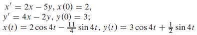
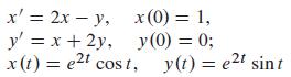
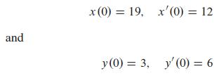
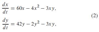
Consider a mass-and-spring system containing two masses m1 = 1 and m2 = 1 whose displacement functions x(t) and y(t) satisfy the differential equations(a) Describe the two fundamental modes of free oscillation of the system.(b) Assume that the two masses start in motion with the initial
In Problems 1 through 10, transform the given differential equation or system into an equivalent system of first-order differential equations.x" = (1 - y)x, y" = (1 - x)y
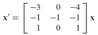
Find general solutions of the systems in Problems 1 through 22. In Problems 1 through 6, use a computer system or graphing calculator to construct a direction field and typical solution curves for the given system. x = 0-4 -1 1 -3 -1 -1 L 1 1 0 X
A computer will be required for the remaining problems in this section. In Problems 9 through 12, an initial value problem and its exact solution are given. In each of these four problems, use the Runge–Kutta method with step sizes h = 0.1 and h = 0.05 to approximate to five decimal places the
Use the method of Examples 5, 6, and 7 to find general solutions of the systems in Problems 11 through 20. If initial conditions are given, find the corresponding particular solution. For each problem, use a computer system or graphing calculator to construct a direction field and typical solution
In Problems 3 through 12, write the given system in the form x' = P(t)x + f(t).x'1 = x2, x'2 = 2x3, x'3 = 3x4, x'4 = 4x1
In Problems 1 through 16, apply the eigenvalue method of this section to find a general solution of the given system. If initial values are given, find also the corresponding particular solution. For each problem, use a computer system or graphing calculator to construct a direction field and
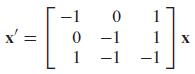
Find general solutions of the systems in Problems 1 through 22. In Problems 1 through 6, use a computer system or graphing calculator to construct a direction field and typical solution curves for the given system. = -1 0 1 0 -1 -1 1 1 -1 X
Use the method of Examples 5, 6, and 7 to find general solutions of the systems in Problems 11 through 20. If initial conditions are given, find the corresponding particular solution. For each problem, use a computer system or graphing calculator to construct a direction field and typical solution
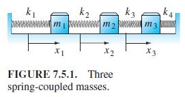
In Problems 12 and 13, find the natural frequencies of the three-mass system of Fig. 7.5.1, using the given masses and spring constants. For each natural frequency ω, give the ratio a1:a2:a3 of amplitudes for a corresponding natural mode x1 = a1 cos ωt , x2 = a2 cos ωt , x3 = a3 cos ωt.m1 = m2
A computer will be required for the remaining problems in this section. In Problems 9 through 12, an initial value problem and its exact solution are given. In each of these four problems, use the Runge–Kutta method with step sizes h = 0.1 and h = 0.05 to approximate to five decimal places the
In Problems 3 through 12, write the given system in the form x' = P(t)x + f(t).x'1 = x2 + x3 + 1, x'2 = x3 + x4 + t, x'3 = x1 + x4 + t2, x'4 = x1 + x2 + t3
In Problems 1 through 16, apply the eigenvalue method of this section to find a general solution of the given system. If initial values are given, find also the corresponding particular solution. For each problem, use a computer system or graphing calculator to construct a direction field and
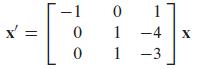
Find general solutions of the systems in Problems 1 through 22. In Problems 1 through 6, use a computer system or graphing calculator to construct a direction field and typical solution curves for the given system. x' = L -1 0 0 0 1 1 1 -4 -3 X
Problems 4 through 7 deal with the competition systemin which c1c2 = 9 > 8 = b1b2, so the effect of competition should exceed that of inhibition. Problems 4 through 7 imply that the four critical points (0,0), (0, 21), (15,0), and (6, 12) of the system in (2) resemble those shown in Fig. 9.3.9-a
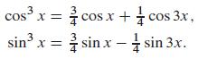
(a) Writeby Euler’s formula, expand, and equate real and imaginary parts to derive the identities(b) Use the result of part (a) to find a general solution of cos 3x + i sin 3x = e3ix = (cos x + i sin x)³
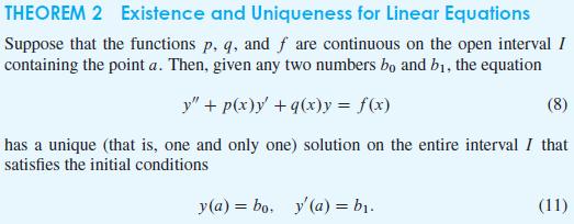
Given a mass m, a dashpot constant c, and a spring constant k, Theorem 2 of Section 5.1 implies that the equationhas a unique solution for t ≧ 0 satisfying given initial conditions x (0) = x0, x'(0) = v0. Thus the future motion of an ideal mass-spring-dashpot system is completely determined by
Use trigonometric identities to find general solutions of the equations in Problems 44 through 46.y'' + y = x cos3 x
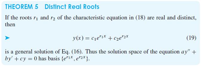
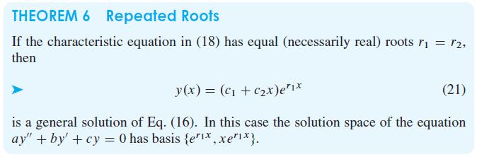
Apply Theorems 5 and 6 to find general solutions of the differential equations given in Problems 33 through 42. Primes denote derivatives with respect to x.y'' + 5y' = 0 THEOREM 5 Distinct Real Roots If the roots ₁ and 2 of the characteristic equation in (18) are real and distinct, then y(x) =

Showing 100 - 200 of 2513

1
2
3
4
5
6
7
8
9
10
11
12
13
14
15
Last

Step by Step Answers

Services

Sitemap
Fun
Definitions
Become Tutor
Used Textbooks
Study Help Categories
Recent Questions
Expert Questions
Campus Wear
Sell Your Books

Company Info

Security
Copyrights
Privacy Policy
Terms & Conditions
SolutionInn Fee
Scholarship
Online Quiz
Give Feedback, Get Rewards

Get In Touch

About Us
Contact Us
Career
Jobs
FAQ
Student Discount
Campus Ambassador

Secure Payment

Download Our App

© 2026 SolutionInn. All Rights Reserved