New Semester Started Get 50% OFF Study Help! --h --m --s Claim Now

Question Answers

Textbooks

Find textbooks, questions and answers

Oops, something went wrong!

Change your search query and then try again

Result Not Found

Books FREE
Study Help
Tutors
AI Study Planner NEW
Sell Books

Search
Sign In
Register

study help
business
elementary statistics

Elementary Statistics 3rd Edition William Navidi, Barry Monk - Solutions

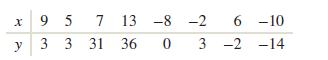
In Exercises 13–16, compute the least-squares regression line for the given data set. x 95 7 y 3 3 31 13-8-2 6-10 36 0 3 3-2-14
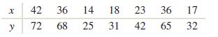
In Exercises 13–16, compute the least-squares regression line for the given data set. x 42 36 14 18 23 36 17 y 72 68 25 31 42 42 65 32
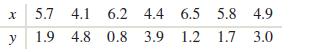
In Exercises 13–16, compute the least-squares regression line for the given data set. x 5.7 5.7 4.1 6.2 4.4 6.5 5.8 4.9 y 1.9 4.8 0.8 3.9 3.9 1.2 1.7 3.0
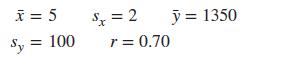
Compute the least-squares regression line for predicting y from x given the following summary statistics: x = 5 Sy = 100 $x = 2 =2 y = 1350 r = 0.70
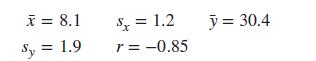
Compute the least-squares regression line for predicting y from x given the following summary statistics: x = 8.1 Sy = 1.9 S. Sx = 1.2 y = 30.4 r = -0.85
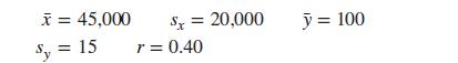
In a hypothetical study of the relationship between the income of parents (x) and the IQs of their children (y), the following summary statistics were obtained:Find the equation of the least-squares regression line for predicting IQ from income. Sx = 20,000 y = 100 x = 45,000 Sy = 15 r = 0.40
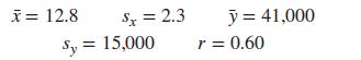
Assume that in a study of educational level in years (x)and income (y), the following summary statistics were obtained:Find the equation of the least-squares regression line for predicting income from educational level. x = 12.8 $x = 2.3 Sy = 15,000 y = 41,000 r = 0.60
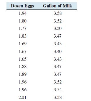
The following table presents the average price in dollars for a dozen eggs and a gallon of milk for each month in a recent year.a. Compute the least-squares regression line for predicting the price of milk from the price of eggs.b. If the price of eggs differs by $0.25 from one month to the next,
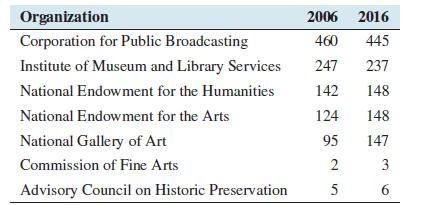
The following table presents the budget (in millions) for selected organizations that received U.S. government funding for arts and culture in both 2006 and 2016.a. Compute the least-squares regression line for predicting the 2016 budget from the 2006 budget.b. If two institutions have budgets that
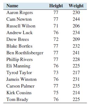
The following table lists the heights (inches) and weights (pounds) of 14 National Football League quarterbacks in the 2016 season.a. Compute the least-squares regression line for predicting weight from height.b. Is it possible to interpret the y-intercept? Explain.c. If two quarterbacks differ in
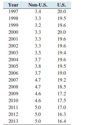
Carbon dioxide (CO2) is produced by burning fossil fuels such as oil and natural gas, and has been connected to global warming. The following table presents the average amounts (in metric tons) of CO2 emissions for the years 1997–2013 per person in the United States and per person in the rest of
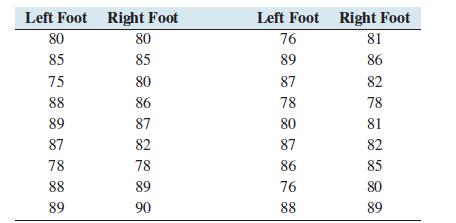
Foot ulcers are a common problem for people with diabetes. Higher skin temperatures on the foot indicate an increased risk of ulcers. In a study carried out at the Colorado School of Mines, skin temperatures on both feet were measured, in degrees Fahrenheit, for 18 diabetic patients. The results
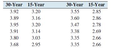
The following table presents interest rates, in percent, for 30-year and 15-year fixed-rate mortgages, for January through December, 2012.a. Compute the least-squares regression line for predicting the 15-year rate from the 30-year rate.b. Construct a scatterplot of the 15-year rate (y) versus the
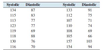
A blood pressure measurement consists of two numbers: the systolic pressure, which is the maximum pressure taken when the heart is contracting, and the diastolic pressure, which is the minimum pressure taken at the beginning of the heartbeat. Blood pressures were measured, in millimeters of mercury
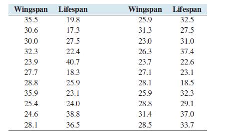
Do larger butterflies live longer? The wingspan (in millimeters) and the lifespan in the adult state (in days) were measured for 22 species of butterfly. Following are the results.a. Compute the least-squares regression line for predicting the lifespan from the wingspan.b. Is it possible to
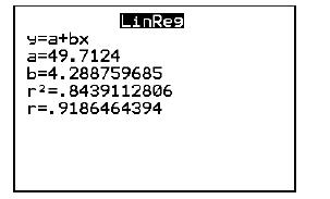
The following display from the TI-84 Plus calculator presents the least-squares regression line for predicting a student’s score on a statistics exam (y) from the number of hours spent studying (x).a. Write the equation of the least-squares regression line.b. What is the correlation between the
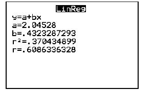
The following display from the TI-84 Plus calculator presents the least-squares regression line for predicting the price of a certain stock (y) from the prime interest rate in percent (x).a. Write the equation of the least-squares regression line.b. What is the correlation between the interest rate
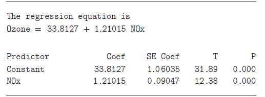
The following MINITAB output presents the least-squares regression line for predicting the concentration of ozone in the atmosphere from the concentration of oxides of nitrogen (NOx).a. Write the equation of the least-squares regression line.b. Predict the ozone concentration when the NOx
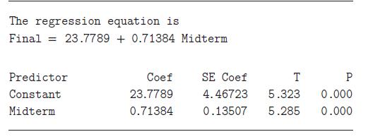
The following MINITAB output presents the least-squares regression line for predicting the score on a final exam from the score on a midterm exam.a. Write the equation of the least-squares regression line.b. Predict the final exam score for a student who scored 75 on the midterm. The regression
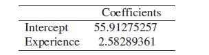
A business school professor computed a least-squares regression line for predicting the salary in $1000s for a graduate from the number of years of experience. The results are presented in the following Excel output.a. Write the equation of the least-squares regression line.b. Predict the salary
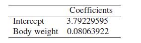
A biologist computed a least-squares regression line for predicting the brain weight in grams of a bird from its body weight in grams. The results are presented in the following Excel output.a. Write the equation of the least-squares regression line.b. Predict the brain weight for a bird whose body
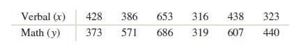
The following table presents math and verbal SAT scores for six freshmen.a. Compute the correlation coefficient between math and verbal SAT score.b. Compute the mean x̄ and the standard deviation sx for the verbal scores.c. Compute the mean ȳ and the standard deviation sy for the math scores.d.
A sample of adults was studied to determine the relationship between education level and annual income. The least-squares regression line for predicting income from education level was computed to be ̂y = 2812 + 3375x, where x is the number of years of education and ̂y is the predicted annual
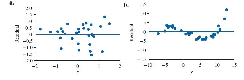
For each of the following residual plots, determine whether a linear model is appropriate. a. b. 15 2.0 10- 1.5 1.0 Residual 0.5 0 Residual -0.5- -1.0 5 0 -5 -10- -1.5- -2.0 -15+ T -2 -1 0 1 2 -10 -5 0 5 10 15 x X
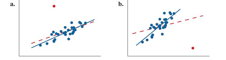
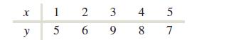
In each of the following plots, one point is an outlier. The blue solid line is the least-squares regression line computed without using the outlier, and the red dashed line is the least-squares regression line computed by including the outlier. State whether the outlier is influential. 2. b.
For each of the following values of the correlation coefficient, determine how much of the variation in the outcome variable is explained by the least-squares regression line.a. r = 0.6b. r = −0.9c. r = 0d. r = 1
5. Making predictions for values of the explanatory variable that are outside of the range of the data is called ____________________ .In Exercises 5–10, fill in each blank with the appropriate word or phrase.
A _________________ is the difference between an observed value and a predicted value of the outcome variable.In Exercises 5–10, fill in each blank with the appropriate word or phrase.
The least-squares property says that the __________________ is smaller for the least-squares regression line than for any other line.In Exercises 5–10, fill in each blank with the appropriate word or phrase.
An outlier that strongly affects the position of a least-squares regression line is said to be ______________________.In Exercises 5–10, fill in each blank with the appropriate word or phrase.
The coefficient of determination is the square of the ____________________ .In Exercises 5–10, fill in each blank with the appropriate word or phrase.
The total variation is the sum of the _____________________ and the __________________ .In Exercises 5–10, fill in each blank with the appropriate word or phrase.
When two values have a nonlinear relationship, the residual plot will exhibit a noticeable pattern.In Exercises 11–14, determine whether the statement is true or false. If the statement is false, rewrite it as a true statement.
When the correlation coefficient is close to 1 or −1, there is not necessarily a linear relationship between the variables.In Exercises 11–14, determine whether the statement is true or false. If the statement is false, rewrite it as a true statement.
The closer r2 is to 0, the closer the predictions made by the least-squares regression line are to the actual values, on average.In Exercises 11–14, determine whether the statement is true or false. If the statement is false, rewrite it as a true statement.
The coefficient of determination may be interpreted as the proportion of variation in the outcome variable explained by the least-squares regression line.In Exercises 11–14, determine whether the statement is true or false. If the statement is false, rewrite it as a true statement.
For the following data set: a. Compute the coefficient of determination.b. How much of the variation in the outcome variable is explained by the least-squares regression line? x y 5 12 6 3. 9 4 5 8 57
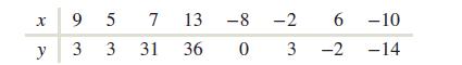
For the following data set:a. Compute the coefficient of determination.b. How much of the variation in the outcome variable is explained by the least-squares regression line? x 95 7 13 -8-2 6-10 y 3 3 31 36 0 3 -2-14
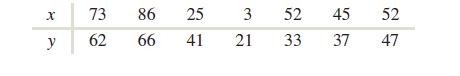
For the following data set:a. Compute the least-squares regression line.b. Which point is an outlier?c. Remove the outlier and compute the least-squares regression line.d. Is the outlier influential? Explain. x 73 86 25 3 52 45 52 y 62 66 41 21 33 37 47
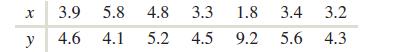
For the following data set:a. Compute the least-squares regression line.b. Which point is an outlier?c. Remove the outlier and compute the least-squares regression line.d. Is the outlier influential? Explain. x 3.9 5.8 4.8 3.3 1.8 3.4 3.2 y 4.6 4.1 5.2 4.5 9.2 5.6 4.3
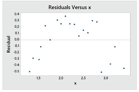
Following is a residual plot produced by MINITAB. Was it appropriate to compute the least-squares regression line? Explain. Residual 0.4 0.3 0.2 Residuals Versus x 0.1 0.0 -0.1 -0.2 -0.3 -0.4 -0.5 1.5 2.0 2.5 3.0 X
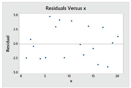
Following is a residual plot produced by MINITAB. Was it appropriate to compute the least-squares regression line? Explain. 00 5.0 2.5 Residual 0.0 -2.5 Residuals Versus x -5.0 -10 5 10 x 15 20 20
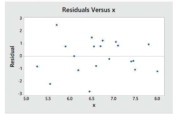
Following is a residual plot produced by MINITAB. Was it appropriate to compute the least-squares regression line? Explain. Residual -2 -3 1 2 3 5.0 5.5 09 6.0 Residuals Versus x 6.5 X 7.0 7.5 8.0
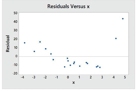
Following is a residual plot produced by MINITAB. Was it appropriate to compute the least-squares regression line? Explain. 50 50 Residuals Versus x 40 40 30 20 20 Residual 10 10 0 -10 -20 20 + -3 -2 2 3 X + 5
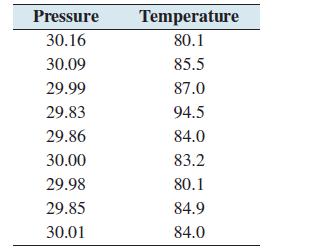
The following table presents the temperature, in degrees Fahrenheit, and barometric pressure, in inches of mercury, on August 15 at 12 noon in Macon, Georgia, over a nine-year period.a. Compute the least-squares regression line for predicting temperature from barometric pressure.b. Compute the
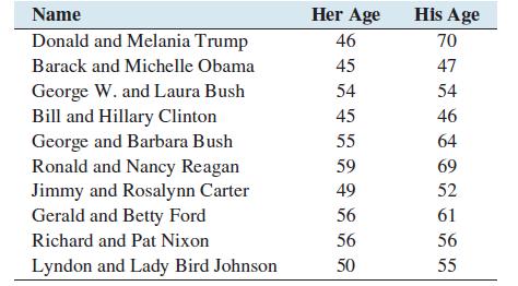
The following table presents the ages of the last 10 U.S. presidents and their wives on the first day of their presidencies.a. Compute the least-squares regression line for predicting the president’s age from the first lady’s age.b. Compute the coefficient of determination.c. Construct a
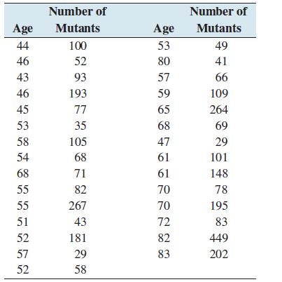
In a study to determine whether the frequency of a certain mutant gene increases with age, the number of mutant genes per microgram of DNA was counted for each of 29 men. The results are presented in the following table.a. Compute the least-squares regression line for predicting number of mutants
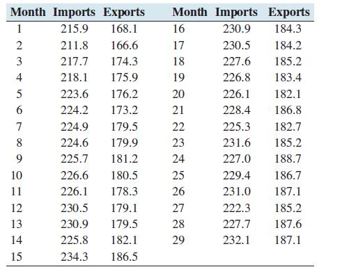
The following table presents the U.S. imports and exports (in billions of dollars) for each of 29 months.a. Compute the least-squares regression line for predicting exports (y) from imports (x).b. Compute the coefficient of determination.c. The months with the two lowest exports are months 1 and 2,
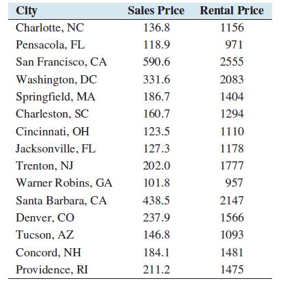
The following table presents the average sales price (in $1000s) and the average monthly rental price of homes in selected U.S. cities in a recent month.a. Compute the least-squares regression line for predicting average rental price (y) from average selling price (x).b. Compute the coefficient of
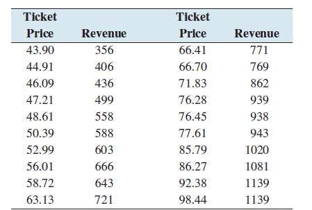
The following table presents the average ticket price (the average price paid per attendee) in dollars and the gross revenue (in millions of dollars) for Broadway productions for each of 20 seasons.a. Compute the least-squares regression line for predicting gross revenue (y) from ticket price
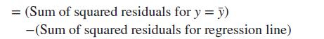
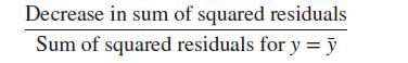
For the house data in Table 4.1, the average selling price is ̄y = 447.0. Imagine that you do not know the size of any house, so you predict the selling price of each of them to be 447.0. This is equivalent to using the line y = ̄y for prediction.a. Compute the residual for each point using the
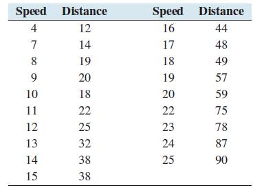
The following table presents the speed (in mph) and the stopping distance (in feet) for a sample of cars.a. Compute the least-squares regression line for predicting stopping distance (y) from speed (x).b. Construct a residual plot. Explain why the least-squares line is not an appropriate summary of
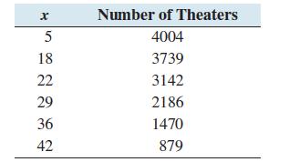
The number of theaters showing the movie Monsters University x days after opening are presented in the following table.Construct a scatterplot with number of days on the horizontal axis and number of theaters on the vertical axis. x Number of Theaters 5 4004 18 3739 22 3142 29 2186 36 1470 42 879
Use the data in Exercise 2 to compute the correlation between the number of days after the opening of the movie and the number of theaters showing the movie. Is the association positive or negative? Weak or strong?Exercise 2The number of theaters showing the movie Monsters University x days after
A scatterplot has a correlation of r = −1. Describe the pattern of the points.
In a survey of U.S. cities, it is discovered that there is a positive correlation between the number of paved streets in the city and the number of registered cars. Does this mean that paving more streets in the city will result in an increase in the number of registered cars? Explain.
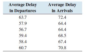
The following table presents the average delay in minutes for departures and arrivals of domestic flights at O’Hare Airport in Chicago for selected years.Compute the least-squares regression line for predicting the delay in arrival time from the delay in departure time. Average Delay in
Use the least-squares regression line computed in Exercise 6 to predict the average delay in arrival time in a year when the average delay in departure time is 58.5 minutes.
Use the least-squares regression line computed in Exercise 6 to compute the residual for the year when the average delay in departure time was 58.4 minutes and the average delay in arrival time was 67.4 minutes.
Refer to Exercise 6.If the average delay in departure times differs by 2 minutes from one year to the next, by how much would you predict the average delay in arrival times to change?Exercise 6The following table presents the average delay in minutes for departures and arrivals of domestic flights
A scatterplot has a least-squares regression line with a slope of 0.What is the correlation coefficient?
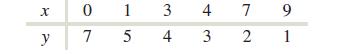
Compute the least-squares regression line for the following data set. x y 17 0 1 3 4 7 9 5 4 3 2 1
Two lines are drawn on a scatterplot. The sum of squared residuals for line A is 558.2, and the sum of squared residuals for line B is 723.1. Which of the following is true about the sum of squared residuals for the least-squares regression line?i. It will be greater than 723.1.ii. It will be
A sample of students was studied to determine the relationship between sleeping habits and classroom performance. The least-squares regression line for predicting the score on a standardized exam from hours of sleep was computed to bêy = 35.6 + 6.8x, where x is the number of hours of sleep and
In a scatterplot, the point (−2, 7) is influential. If this point is removed from the scatterplot, which of the following describes the effect on the least-squares regression line?i. It will shift its position by a substantial amount.ii. It will shift its position slightly.iii. It will not shift
The correlation coefficient for a data set is r = −0.6. How much of the variation in the outcome variable is explained by the least-squares regression line?
Describe an example in which two variables are strongly correlated, but changes in one do not cause changes in the other.
Explain why the predicted value ̂y is always equal to ̄y when r = 0.
Describe conditions under which the slope of the least-squares line will be equal to the correlation coefficient.
Describe circumstances under which the sum of the squared residuals will equal zero. What conclusions can be drawn about the least-squares regression line in this case?
Explain why extrapolation may lead to unreliable results.
Explain how it is possible for a point to be an outlier without being an influential point.
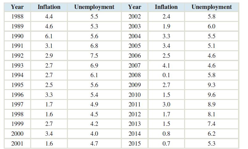
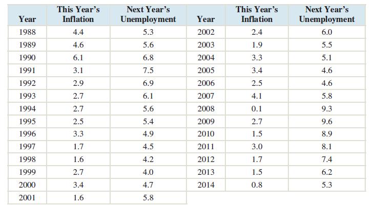
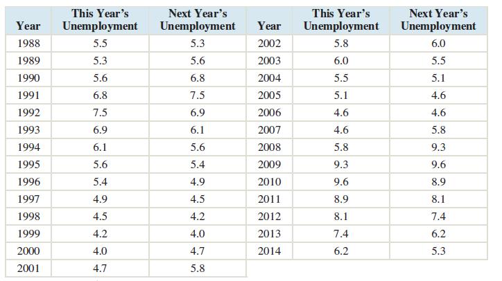
1. The following table, reproduced from the chapter introduction, presents the inflation rate and unemployment rate, both in percent, for the years 1988–2015.We will investigate some methods for predicting unemployment. First, we will try to predict the unemployment rate from the inflation
The population of country A is twice as large as the population of country B. True or false: If images are used to represent the populations, both the height and width of the image for country A should be twice as large as the height and width of the image for country B.
If the baseline of a bar graph or time-series plot is not at zero, then the differences may appear to be __________________ than they actually are.
A plot that represents how much of something there is may be misleading if the baseline is not at ______________________.In Exercises 3 and 4, fill in each blank with the appropriate word or phrase.
The area principle says that when images are used to compare amounts, the areas of the images should be ______________________ to the amounts.In Exercises 3 and 4, fill in each blank with the appropriate word or phrase.
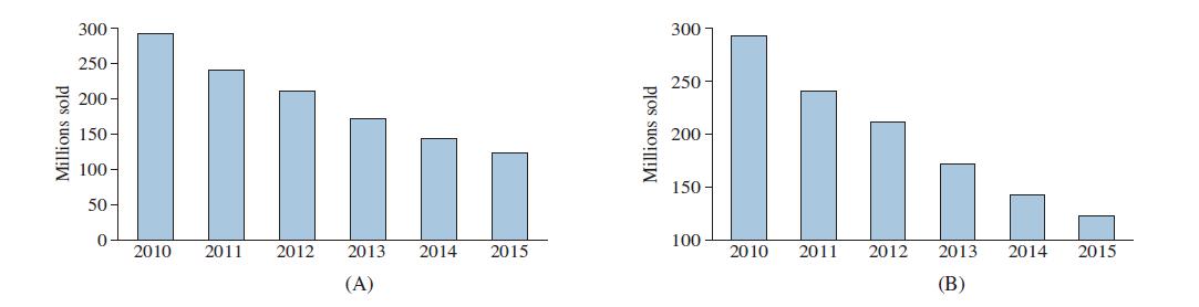
Sales of CDs have been declining for several years as more music is downloaded over the Internet. Following are two bar graphs that illustrate the decline in CD sales. (Source: Recording Industry Association of America)Choose one of the following options, and explain why it is correct:(i) Graph A
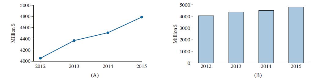
The following time-series plot and bar graph both present the sales of digital music for the years 2012–2015. Which of the graphs presents the more accurate picture? Why? Million $ 5000 4800- 5000 4000 3000 4600 4400 Million $ 2000 4200 1000 4000 2012 0 2013 2014 2015 2012 2013 2014 2015 (A) (B)
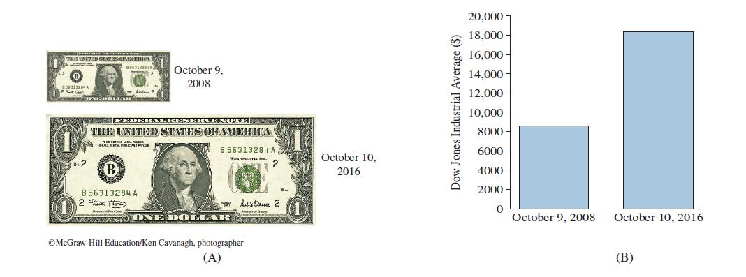
The Dow Jones Industrial Average reached its lowest point in recent history on October 9, 2008, when it closed at$8,579. Eight years later, on October 10, 2016, the average had risen to $18,329.04.Which of the following graphs accurately represents the magnitude of the increase? Which one
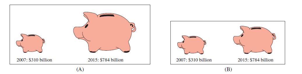
In 2007, U.S. residents saved approximately $310 billion. In 2015, that amount was $784 billion, about two-and-a-half times greater. Which of the following graphs compares these totals more accurately, and why? 2007: $310 billion 2015: $784 billion 2007: $310 billion 2015: $784 billion (A) (B)
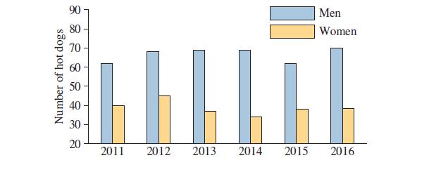
The following bar graph presents the number of hot dogs eaten by the men’s and women’s winner of Nathan’s Famous Hot Dog eating championship for the years 2011–2016. Does the graph present an accurate picture of the difference between the men’s and women’s winners? Or is it misleading?
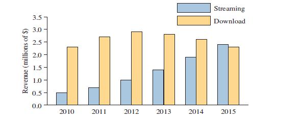
The following bar graph presents the revenue (in millions of $) for the music industry from music streaming and music downloading for the years 2010–2015. Does the graph present an accurate picture of the differences in revenue from these two sources? Or is it misleading? Explain Revenue
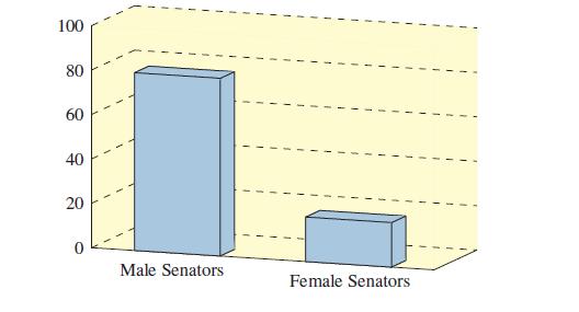
Of the 100 members of the United States Senate recently, 80 were men and 20 were women. The following three-dimensional bar graph attempts to present this information.a. Explain how this graph is misleading.b. Construct a graph (not necessarily three-dimensional) that presents this information
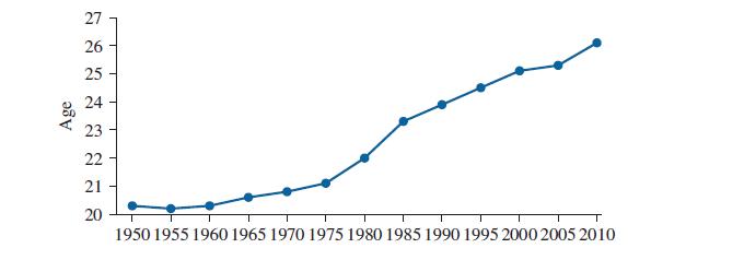
Data compiled by the U.S. Census Bureau suggests that the age at which women first marry has increased over time. The following time-series plot presents the average age at which women first marry for the years 1950–2010. Does the plot present an accurate picture of the increase, or is it
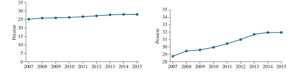
Both of the following time-series plots present the percentage of U.S. adults who have earned college degrees during the years 2007–2015.Which of the following statements is true and why?i. The percentage of U.S. adults with college degrees increased slightly between 2007 and 2015.ii. The
Both of the following time-series plots present the percentage of income spent on food by U.S. residents for the years 1998 through 2014. Which of the following statements is more accurate, and why?(i) The percentage of income spent on food decreased considerably between 1998 and 2014.(ii) The
Following is the list of letter grades for students in an algebra class: A, B, F, A, C, C, A, B, D, F, D, A, A, B, C, F, B, D, C, A, A, A, F, B, C, A, C. Construct a frequency distribution for these data.
Construct a relative frequency distribution for the data in Exercise 1.Exercise 1 Following is the list of letter grades for students in an algebra class: A, B, F, A, C, C, A, B, D, F, D, A, A, B, C, F, B, D, C, A, A, A, F, B, C, A, C. Construct a frequency distribution for these data.
Construct a frequency bar graph for the data in Exercise 1.Exercise 1 Following is the list of letter grades for students in an algebra class: A, B, F, A, C, C, A, B, D, F, D, A, A, B, C, F, B, D, C, A, A, A, F, B, C, A, C. Construct a frequency distribution for these data.
Construct a pie chart for the data in Exercise 1.Exercise 1 Following is the list of letter grades for students in an algebra class: A, B, F, A, C, C, A, B, D, F, D, A, A, B, C, F, B, D, C, A, A, A, F, B, C, A, C. Construct a frequency distribution for these data.
The first class in a relative frequency distribution is 2.0–4.9, and there are six classes. Find the remaining five classes.What is the class width?
True or false: A histogram can have more than one mode.
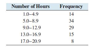
A sample of 100 students was asked how many hours per week they spent studying. The following frequency distribution shows the results.a. Construct a frequency histogram for these data.b. Construct a relative frequency histogram for these data. Number of Hours Frequency 1.0-4.9 14 5.0-8.9 34
Construct a frequency polygon for the data in Exercise 7.Exercise 7 A sample of 100 students was asked how many hours per week they spent studying. The following frequency distribution shows the results. Number of Hours Frequency 1.0-4.9 14 5.0-8.9 34 9.0-12.9 29 13.0-16.9 15 17.0-20.9 8
Construct a relative frequency ogive for the data in Exercise 7.Exercise 7 A sample of 100 students was asked how many hours per week they spent studying. The following frequency distribution shows the results. Number of Hours Frequency 1.0-4.9 14 5.0-8.9 34 9.0-12.9 29 13.0-16.9 15 17.0-20.9 8
Following are the prices (in dollars) for a sample of coffee makers.Construct a stem-and-leaf plot for these data. 19 22 29 68 35 37 28 22 41 39 28
Following are the prices (in dollars) for a sample of espresso makers.Construct a back-to-back stem-and-leaf plot for these data and the data in Exercise 11.Exercise 11Following are the prices (in dollars) for a sample of coffee makers.Construct a stem-and-leaf plot for these data. 99 99 50 50 31
Construct a dotplot for the data in Exercise 11.Exercise 11Following are the prices (in dollars) for a sample of coffee makers.Construct a stem-and-leaf plot for these data. 19 22 29 68 35 37 28 22 41 39 28
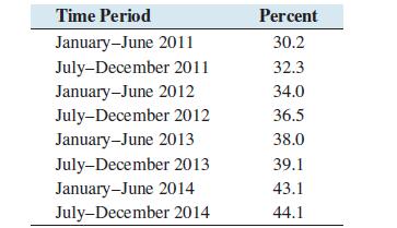
The following table presents the percentage of Americans who use a cell phone exclusively, with no landline phone, for the years 2011–2014. Construct a time-series plot for these data. Time Period January-June 2011 Percent 30.2 July-December 2011 32.3 January-June 2012 34.0 July-December 2012

Showing 7100 - 7200 of 7930

First
65
66
67
68
69
70
71
72
73
74
75
76
77
78
79
Last

Step by Step Answers

Services

Sitemap
Fun
Definitions
Become Tutor
Used Textbooks
Study Help Categories
Recent Questions
Expert Questions
Campus Wear
Sell Your Books

Company Info

Security
Copyrights
Privacy Policy
Terms & Conditions
SolutionInn Fee
Scholarship
Online Quiz
Give Feedback, Get Rewards

Get In Touch

About Us
Contact Us
Career
Jobs
FAQ
Student Discount
Campus Ambassador

Secure Payment

Download Our App

© 2026 SolutionInn. All Rights Reserved