New Semester
Started
Get
50% OFF
Study Help!
--h --m --s
Claim Now
Question Answers
Textbooks
Find textbooks, questions and answers
Oops, something went wrong!
Change your search query and then try again
S
Books
FREE
Study Help
Expert Questions
Accounting
General Management
Mathematics
Finance
Organizational Behaviour
Law
Physics
Operating System
Management Leadership
Sociology
Programming
Marketing
Database
Computer Network
Economics
Textbooks Solutions
Accounting
Managerial Accounting
Management Leadership
Cost Accounting
Statistics
Business Law
Corporate Finance
Finance
Economics
Auditing
Tutors
Online Tutors
Find a Tutor
Hire a Tutor
Become a Tutor
AI Tutor
AI Study Planner
NEW
Sell Books
Search
Search
Sign In
Register
study help
mathematics
elementary statistics picturing
Elementary Statistics Picturing The World 7th Edition Ron Larson, Betsy Farber - Solutions
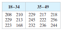
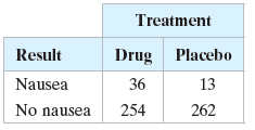
The table at the left shows a sample of the waiting times (in days) for a heart transplant for two age groups. At a = 0.05, can you conclude that the variances of the waiting times differ between the two age groups?(a) Identify the claim and state H0 and Ha, (b) Find the critical value and
Find the critical F-value for a two-tailed test using the level of significance α and degrees of freedom d.f.N and d.f.D.α = 0.05, d.f. N = 27, d.f.D = 19
Find the critical F-value for a two-tailed test using the level of significance α and degrees of freedom d.f.N and d.f.D.α = 0.05, d.f. N = 60, d.f.D = 40
Find the critical F-value for a two-tailed test using the level of significance α and degrees of freedom d.f.N and d.f.D.α = 0.10, d.f. N = 24, d.f.D = 28
Find the critical F-value for a two-tailed test using the level of significance α and degrees of freedom d.f.N and d.f.D.α = 0.01, d.f.N = 6, d.f.D = 7
Find the critical F-value for a right-tailed test using the level of significance a and degrees of freedom d.f.N and d.f.D.α = 0.025, d.f. N = 7, d.f.D = 3
Find the critical F-value for a right-tailed test using the level of significance a and degrees of freedom d.f.N and d.f.D.α = 0.10, d.f. N = 10, d.f. D = 15
Find the critical F-value for a right-tailed test using the level of significance a and degrees of freedom d.f.N and d.f.D.α = 0.01, d.f. N = 2, d.f. D = 11
Find the critical F-value for a right-tailed test using the level of significance a and degrees of freedom d.f.N and d.f.D.α = 0.05, d.f.N = 9, d.f. D = 16
List the three conditions that must be met in order to use a two-sample F-test.
Explain how to find the critical value for an F-test.
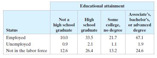
What percent of U.S. adults ages 25 and over who are not high school graduates are unemployed?Use the contingency table, and the information below. Relative frequencies can also be calculated based on the row totals (by dividing each row entry by the row’s total) or the column totals (by dividing
What percent of U.S. adults ages 25 and over who have a degree are not in the labor force?Use the contingency table, and the information below. Relative frequencies can also be calculated based on the row totals (by dividing each row entry by the row’s total) or the column totals (by dividing
Calculate the conditional relative frequencies in the contingency table based on the column totals.Use the contingency table, and the information below. Relative frequencies can also be calculated based on the row totals (by dividing each row entry by the row’s total) or the column totals (by
What percent of U.S. adults ages 25 and over who are not in the labor force have some college education, but no degree?Use the contingency table, and the information below. Relative frequencies can also be calculated based on the row totals (by dividing each row entry by the row’s total) or the
What percent of U.S. adults ages 25 and over who are employed have a degree?Use the contingency table, and the information below. Relative frequencies can also be calculated based on the row totals (by dividing each row entry by the row’s total) or the column totals (by dividing each column entry
Calculate the conditional relative frequencies in the contingency table based on the row totals.Use the contingency table, and the information below. Relative frequencies can also be calculated based on the row totals (by dividing each row entry by the row’s total) or the column totals (by
What percent of U.S. adults ages 25 and over (a) Are employed and are only high school graduates, (b) Are not in the labor force, and (c) Are not high school graduates?Use the information below. The frequencies in a contingency table can be written as relative frequencies by
What percent of U.S. adults ages 25 and over (a) Have a degree and are unemployed and (b) Have some college education, but no degree, and are not in the labor force?Use the information below. The frequencies in a contingency table can be written as relative frequencies by dividing
Explain why you cannot perform the chi-square independence test on these data.Use the information below. The frequencies in a contingency table can be written as relative frequencies by dividing each frequency by the sample size. The contingency table below shows the number of U.S. adults (in
Rewrite the contingency table using relative frequencies.Use the information below. The frequencies in a contingency table can be written as relative frequencies by dividing each frequency by the sample size. The contingency table below shows the number of U.S. adults (in millions) ages 25 and
Is the chi-square homogeneity of proportions test a left-tailed, right-tailed, or two-tailed test?
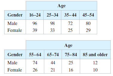
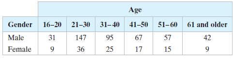
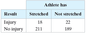
The contingency table shows the results of a random sample of motor vehicle crash deaths by age and gender. At α = 0.05, perform a homogeneity of proportions test on the claim that the proportions of motor vehicle crash deaths involving males or females are the same for each age group. Age Gender
Use the contingency table and expected frequencies from Exercise 12. At α = 0.10, test the hypothesis that the variables are dependent.Perform the indicated chi-square independence test by performing the steps below.(a) Identify the claim and state H0 and Ha.(b) Determine the degrees of freedom,
Use the contingency table and expected frequencies from Exercise 11. At α = 0.10, test the hypothesis that the variables are independent.Perform the indicated chi-square independence test by performing the steps below.(a) Identify the claim and state H0 and Ha.(b) Determine the degrees of freedom,
Use the contingency table and expected frequencies from Exercise 10. At α = 0.01, test the hypothesis that the variables are dependent.Perform the indicated chi-square independence test by performing the steps below.(a) Identify the claim and state H0 and Ha.(b) Determine the degrees of freedom,
Use the contingency table and expected frequencies from Exercise 9. At a = 0.05, test the hypothesis that the variables are dependent.Perform the indicated chi-square independence test by performing the steps below.(a) Identify the claim and state H0 and Ha.(b) Determine the degrees of freedom,
The contingency table shows the results of a random sample of fatally injured passenger vehicle drivers (with blood alcohol concentrations greater than or equal to 0.08) by age and gender. At α = 0.05, can you conclude that age is related to gender in such alcohol-related accidents?Perform the
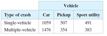
You work for an insurance company and are studying the relationship between types of crashes and the vehicles involved in passenger vehicle occupant deaths. As part of your study, you randomly select 4270 vehicle crashes and organize the resulting data as shown in the contingency table. At α =
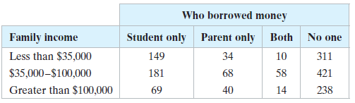
A financial aid officer is studying the relationship between who borrows money to pay for college in a family and the income of the family. As part of the study, 1593 families are randomly selected and the resulting data are organized as shown in the contingency table. At α = 0.01, can you
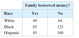
The contingency table shows a random sample of white, black, and Hispanic college students based on whether their family borrowed money to pay for their college education. At α = 0.01, can you conclude that borrowing money for college and race are related?Perform the indicated chi-square
Use the contingency table and expected frequencies from Exercise 8. At α = 0.05, test the hypothesis that the variables are dependent.Perform the indicated chi-square independence test by performing the steps below.(a) Identify the claim and state H0 and Ha.(b) Determine the degrees of freedom,
Use the contingency table and expected frequencies from Exercise 7. At α = 0.01, test the hypothesis that the variables are independent.Perform the indicated chi-square independence test by performing the steps below.(a) Identify the claim and state H0 and Ha.(b) Determine the degrees of freedom,
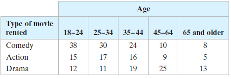
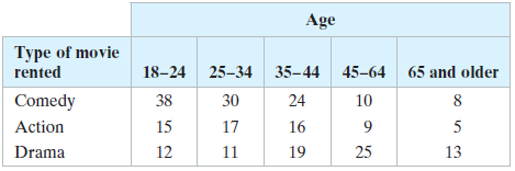
(a) Calculate the marginal frequencies and (b) Find the expected frequency for each cell in the contingency table. Assume that the variables are independent. Age Type of movie rented 45-64 65 and older 18-24 35-44 25-34 24 16 38 30 10 Comedy Action Drama 15 17 5 19 25 13 12 11
When the test statistic for the chi-square independence test is large, you will, in most cases, reject the null hypothesis.Determine whether the statement is true or false. If it is false, rewrite it as a true statement.
If the two variables in a chi-square independence test are dependent, then you can expect little difference between the observed frequencies and the expected frequencies.Determine whether the statement is true or false. If it is false, rewrite it as a true statement.
Explain why the chi-square independence test is always a right-tailed test.
Explain the difference between marginal frequencies and joint frequencies in a contingency table.
Explain how to find the expected frequency for a cell in a contingency table.
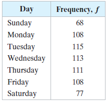
A doctor claims that the number of births by day of the week is uniformly distributed. To test this claim, you randomly select 700 births from a recent year and record the day of the week on which each takes place. The table shows the results. At α = 0.10, test the doctor’s claim.(a) Identify
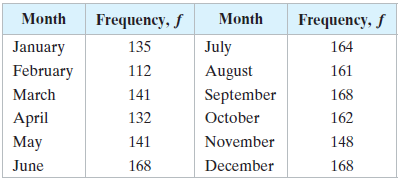
A researcher claims that the number of homicide crimes in California by month is uniformly distributed. To test this claim, you randomly select 1800 homicides from a recent year and record the month when each happened. The table shows the results. At α = 0.10, test the researcher’s claim.(a)
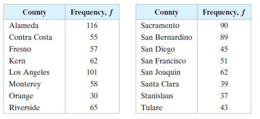
A researcher claims that the number of homicide crimes in California by county is uniformly distributed. To test this claim, you randomly select 1000 homicides from a recent year and record the county in which each happened. The table shows the results. At α = 0.01, test the researcher’s
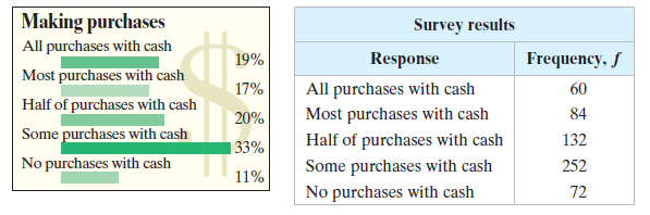
A financial analyst claims that the distribution of people who use cash to make their purchases is different from the distribution shown in the figure. You randomly select 600 people and record the way they make purchases. The table shows the results. At α = 0.01, test the financial analyst’s
n = 415, pi = 0.08Find the expected frequency for the values of n and pi.
n = 230, pi = 0.25Find the expected frequency for the values of n and pi.
n = 500, pi = 0.9Find the expected frequency for the values of n and pi.
Find the expected frequency for the values of n and pi.n = 150, pi = 0.3
What conditions are necessary to use the chi-square goodness-of-fit test?
The equation used to predict the stock price (in dollars) at the end of the year for a restaurant chain isŷ = -86 + 7.46x1 - 1.61x2where x1 is the total revenue (in billions of dollars) and x2 is the shareholders’ equity (in billions of dollars). Use the multiple regression equation to predict
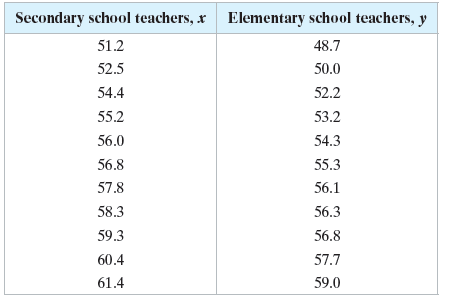
Construct a 95% prediction interval for the average annual salary of elementary school teachers when the average annual salary of secondary school teachers is $52,500. Interpret the results.Use the data in the table, which shows the average annual salaries (both in thousands of dollars) for
Find the standard error of estimate se and interpret the result.Use the data in the table, which shows the average annual salaries (both in thousands of dollars) for secondary and elementary school teachers, excluding special and vocational education teachers, in the United States for 11 years.
Find the coefficient of determination r2 and interpret the result.Use the data in the table, which shows the average annual salaries (both in thousands of dollars) for secondary and elementary school teachers, excluding special and vocational education teachers, in the United States for 11 years.
Use the regression equation that you found in Exercise 4 to predict the average annual salary of elementary school teachers when the average annual salary of secondary school teachers is $52,500.Use the data in the table, which shows the average annual salaries (both in thousands of dollars) for
Find the equation of the regression line for the data. Draw the regression line on the scatter plot that you constructed in Exercise 1.Use the data in the table, which shows the average annual salaries (both in thousands of dollars) for secondary and elementary school teachers, excluding special
Test the significance of the correlation coefficient r that you found in Exercise 2. Use α = 0.05.Use the data in the table, which shows the average annual salaries (both in thousands of dollars) for secondary and elementary school teachers, excluding special and vocational education teachers, in
Calculate the correlation coefficient r and interpret the result.Use the data in the table, which shows the average annual salaries (both in thousands of dollars) for secondary and elementary school teachers, excluding special and vocational education teachers, in the United States for 11 years.
Construct a scatter plot for the data. Do the data appear to have a positive linear correlation, a negative linear correlation, or no linear correlation? Explain.Use the data in the table, which shows the average annual salaries (both in thousands of dollars) for secondary and elementary school
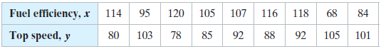
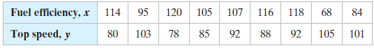
Construct a 99% prediction interval for the top speed of a hybrid or electric car in Exercise 17 that has a combined city and highway fuel economy of 90 miles per gallon equivalentConstruct the indicated prediction interval and interpret the results.Data from Exercise 17:The table shows the
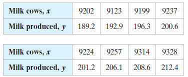
Construct a 90% prediction interval for the amount of milk produced in Exercise 9 when there are an average of 9275 milk cows.Construct the indicated prediction interval and interpret the results.Data from Exercise 9:The average number (in thousands) of milk cows and the amounts (in billions of
The table shows the cooking areas (in square inches) of 18 gas grills and their prices (in dollars). The regression equation is ŷ = 2.335x - 853.278.Use the data to (a) Find the coefficient of determination r2 and interpret the result, and(b) find the standard error of estimate se and
The table shows the combined city and highway fuel efficiency (in miles per gallon gasoline equivalent) and top speeds (in miles per hour) for nine hybrid and electric cars. The regression equation is ŷ = -0.465x + 139.433.Use the data to (a) Find the coefficient of determination r2 and
Use the value of the correlation coefficient r to calculate the coefficient of determination r2. What does this tell you about the explained variation of the data about the regression line? about the unexplained variation?r = 0.795
Use the value of the correlation coefficient r to calculate the coefficient of determination r2. What does this tell you about the explained variation of the data about the regression line? about the unexplained variation?r = 0.642
Use the value of the correlation coefficient r to calculate the coefficient of determination r2. What does this tell you about the explained variation of the data about the regression line? about the unexplained variation?r = -0.937
Use the value of the correlation coefficient r to calculate the coefficient of determination r2. What does this tell you about the explained variation of the data about the regression line? about the unexplained variation?r = -0.450
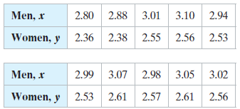
The average times (in hours) per day spent watching television for men and women for 10 years.(a) x = 2.85 hours (b) x = 2.97 hours(c) x = 3.04 hours (d) x = 3.13 hoursFind the equation of the regression line for the data. Then construct a scatter plot of the data and draw the regression
The average number (in thousands) of milk cows and the amounts (in billions of pounds) of milk produced in the United States for eight years.(a) x = 9080 cows (b) x = 9230 cows(c) x = 9250 cows (d) x = 9300 cowsFind the equation of the regression line for the data. Then construct a
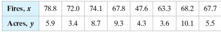
The numbers of wildland fires (in thousands) and wildland acres burned (in millions) in the United States for eight years.(a) Display the data in a scatter plot, (b) Calculate the sample correlation coefficient r, and (c) Describe the type of correlation and interpret the correlation in
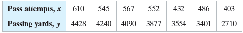
The numbers of pass attempts and passing yards for seven professional quarterbacks for a recent regular season.(a) Display the data in a scatter plot, (b) Calculate the sample correlation coefficient r, and (c) Describe the type of correlation and interpret the correlation in the context
In Exercise 59, is there enough evidence to reject the claim at the α = 0.01 level? Explain.Data from Exercise 59;A bolt manufacturer makes a type of bolt to be used in airtight containers. The manufacturer claims that the variance of the bolt widths is at most 0.01. A random sample of 28 bolts
In Exercise 60, is there enough evidence to reject the claim at the α = 0.05 level? Explain.Data from Exercise 60:A restaurant claims that the standard deviation of the lengths of serving times is 3 minutes. A random sample of 27 serving times has a standard deviation of 3.9 minutes. At a = 0.01,
Find the critical value(s) and rejection region(s) for the type of chi-square test with sample size n and level of significance α.Left-tailed test, n = 6, α = 0.05
Find the critical value(s) and rejection region(s) for the type of chi-square test with sample size n and level of significance α.Two-tailed test, n = 41, α = 0.10
Find the critical value(s) and rejection region(s) for the type of chi-square test with sample size n and level of significance α.Two-tailed test, n = 14, α = 0.01
Find the critical value(s) and rejection region(s) for the type of chi-square test with sample size n and level of significance α.Right-tailed test, n = 20, α = 0.05
A labor researcher claims that 6% of U.S. employees say it is likely they will be laid off in the next year. In a random sample of 547 U.S. employees, 44 said it is likely they will be laid off in the next year. At α = 0.05, is there enough evidence to reject the researcher’s claim?(a) Identify
A polling agency reports that over 40% of U.S. adults say they are less likely to travel to Europe in the next six months for fear of terrorist attacks. In a random sample of 1000 U.S. adults, 42% said they are less likely to travel to Europe in the next six months for fear of terrorist attacks. At
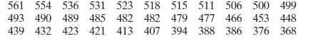
An education researcher claims that the overall average score of 15-year-old students on an international mathematics literacy test is 494. You want to test this claim. You randomly select the average scores of 33 countries. The results are listed below. At α = 0.05, do you have enough evidence to
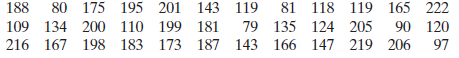
An education publication claims that the mean score for grade 12 students on a science achievement test is more than 145. You want to test this claim. You randomly select 36 grade 12 test scores. The results are listed below. At α = 0.1, can you support the publication’s claim?(a) Identify the
Test the claim about the population mean m at the level of significance a. Assume the population is normally distributed.Claim: μ ≠ 3,330,000; α = 0.05.Sample statistics: x̅ = 3,293,995, s = 12,801, n = 35
Test the claim about the population mean m at the level of significance a. Assume the population is normally distributed.Claim: μ = 195; α = 0.10. Sample statistics: x̅ = 190, s = 36, n = 101
Find the critical value(s) and rejection region(s) for the type of t-test with level of significance a and sample size n.Two-tailed test, α = 0.02, n = 12
Find the critical value(s) and rejection region(s) for the type of t-test with level of significance a and sample size n.Left-tailed test, α = 0.005, n = 15
Find the critical value(s) and rejection region(s) for the type of t-test with level of significance a and sample size n.Left-tailed test, α = 0.05, n = 48
Find the critical value(s) and rejection region(s) for the type of t-test with level of significance a and sample size n.Right-tailed test, α = 0.02, n = 63
Find the critical value(s) and rejection region(s) for the type of t-test with level of significance a and sample size n.Right-tailed test, α = 0.01, n = 33
Find the critical value(s) and rejection region(s) for the type of t-test with level of significance a and sample size n.Two-tailed test, α = 0.05, n = 20
A travel analyst claims that the mean price of a round trip flight from New York City to Los Angeles is less than $507. In a random sample of 55 round trip flights from New York City to Los Angeles, the mean price is $502. Assume the population standard deviation is $111. At α = 0.05, is there
An environmental researcher claims that the mean amount of sulfur dioxide in the air in U.S. cities is 1.15 parts per billion. In a random sample of 134 U.S. cities, the mean amount of sulfur dioxide in the air is 0.93 parts per billion. Assume the population standard deviation is 2.62 parts per
A researcher claims that the mean annual consumption of cotton is greater than 1.1 million bales per country. A random sample of 67 countries has a mean annual consumption of 1.0 million bales. Assumethe population standard deviation is 4.3 million bales. At α = 0.01, can you support the claim?(a)
A researcher claims that the mean annual production of cotton is 3.5 million bales per country. A random sample of 44 countries has a mean annual production of 2.1 million bales. Assume the population standard deviation is 4.5 million bales. At α = 0.05, can you reject the claim?(a) Identify the
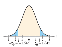
State whether the standardized test statistic z allows you to reject the null hypothesis. Explain your reasoning.z = -1.655 -3 -2 |-1 -20 =-1.645 2 1.645 Zo
State whether the standardized test statistic z allows you to reject the null hypothesis. Explain your reasoning.z = -1.464 -3 -2 |-1 -20 =-1.645 2 1.645 Zo
State whether the standardized test statistic z allows you to reject the null hypothesis. Explain your reasoning.z = 1.723 -3 -2 |-1 -20 =-1.645 2 1.645 Zo
State whether the standardized test statistic z allows you to reject the null hypothesis. Explain your reasoning.z = 1.631 -3 -2 |-1 -20 =-1.645 2 1.645 Zo
Find the P-value for the hypothesis test with the standardized test statistic z. Decide whether to reject H0 for the level of significance α.Two-tailed test, z = 2.57, α = 0.10
Find the P-value for the hypothesis test with the standardized test statistic z. Decide whether to reject H0 for the level of significance α.Left-tailed test, z = -0.94, α = 0.05
A nonprofit consumer organization says that the standard deviation of the fuel economies of its top-rated vehicles for a recent year is no more than 9.5 miles per gallon.(a) State the null and alternative hypotheses and identify which represents the claim, (b) Describe type I and type II
A polling organization reports that the proportion of U.S. adults who have volunteered their time or donated money to help clean up the environment is 65%.(a) State the null and alternative hypotheses and identify which represents the claim, (b) Describe type I and type II errors for a
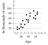
The scatter plots show the results of a survey of 20 randomly selected males ages 24 –35. Using age as the explanatory variable, match each graph with the appropriate description. Explain your reasoning.(a) Age and body temperature (b) Age and balance on student loans(c) Age and
Showing 1500 - 1600
of 2934
First
9
10
11
12
13
14
15
16
17
18
19
20
21
22
23
Last
Step by Step Answers