New Semester Started Get 50% OFF Study Help! --h --m --s Claim Now

Question Answers

Textbooks

Find textbooks, questions and answers

Oops, something went wrong!

Change your search query and then try again

Result Not Found

Books FREE
Study Help
Tutors
AI Study Planner NEW
Sell Books

Search
Sign In
Register

study help
mathematics
statistics the art and science

Statistics Unlocking The Power Of Data 1st Edition Robin H. Lock, Patti Frazer Lock, Kari Lock Morgan, Eric F. Lock, Dennis F. Lock - Solutions

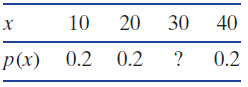
Fill in the ? to make p(x) a probability function. If not possible, say so. 40 10 30 х p(x) 0.2 0.2 0.2
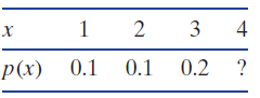
Fill in the ? to make p(x) a probability function. If not possible, say so. 4 х 3 p(x) 0.1 0.1 0.2 ?
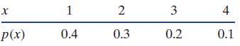
Find P(X is an even number).Refer to the probability function given in Table 11.10 for a random variable X that takes on the values 1, 2, 3, and 4.Table 11.10 2 4 3 0.1 P(x) 0.2 0.4 0.3
Find P(X is an odd number).Refer to the probability function given in Table 11.10 for a random variable X that takes on the values 1, 2, 3, and 4.Table 11.10 2 4 3 0.1 P(x) 0.2 0.4 0.3
Find P(X < 3).Refer to the probability function given in Table 11.10 for a random variable X that takes on the values 1, 2, 3, and 4.Table 11.10 2 4 3 0.1 P(x) 0.2 0.4 0.3
Find P(X > 1).Refer to the probability function given in Table 11.10 for a random variable X that takes on the values 1, 2, 3, and 4.Table 11.10 2 4 3 0.1 P(x) 0.2 0.4 0.3
Find P(X = 3 or X = 4).Refer to the probability function given in Table 11.10 for a random variable X that takes on the values 1, 2, 3, and 4.Table 11.10 2 4 3 0.1 P(x) 0.2 0.4 0.3
Verify that the values given in Table 11.10 meet the conditions for being a probability function. Justify your answer.Refer to the probability function given in Table 11.10 for a random variable X that takes on the values 1, 2, 3, and 4.Table 11.10 2 4 3 0.1 P(x) 0.2 0.4 0.3
Observe the average weight, in pounds, of everything you catch during a day of fishing.State whether the process described is a discrete random variable, is a continuous random variable, or is not a random variable.
Deal cards one at a time from a deck. Keep going until you deal an ace. Stop and count the total number of cards dealt.State whether the process described is a discrete random variable, is a continuous random variable, or is not a random variable.
Draw one M&M from a bag. Observe whether it is blue, green, brown, orange, red, or yellow.State whether the process described is a discrete random variable, is a continuous random variable, or is not a random variable.
Draw 10 cards from a deck and find the proportion that are hearts.State whether the process described is a discrete random variable, is a continuous random variable, or is not a random variable.
Draw 10 cards from a deck and count the number of hearts.State whether the process described is a discrete random variable, is a continuous random variable, or is not a random variable.
Given that a message contains the word ‘‘free” but does NOT contain the word ‘‘text” (or ‘‘txt”), what is the probability that it is spam?Refer to a large collection of real SMS text messages from participating cellphone users.13 In this collection, 747 of the 5574 total messages
Of all spam messages, 17.00% contain both the word ‘‘free” and the word ‘‘text” (or ‘‘txt”). For example, ‘‘Congrats!! You are selected to receive a free camera phone, txt ******* to claim your prize.” Of all non-spam messages, 0.06% contain both the word ‘‘free” and
The word ‘‘text” (or ‘‘txt”) is contained in 7.01% of all messages, and in 38.55% of all spam messages. What is the probability that a message is spam, given that it contains the word ‘‘text” (or ‘‘txt”)?Refer to a large collection of real SMS text messages from
The word ‘‘free” is contained in 4.75% of all messages, and 3.57% of all messages both contain the word ‘‘free” and are marked as spam.(a) What is the probability that a message contains the word ‘‘free”, given that it is spam?(b) What is the probability that a message is spam,
Slippery Elum is a baseball pitcher who uses three pitches, 60% fastballs, 25% curveballs, and the rest spitballs. Slippery is pretty accurate with his fastball (about 70% are strikes), less accurate with his curveball (50% strikes), and very wild with his spitball (only 30% strikes). Slippery ends
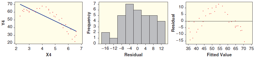
Three graphs are shown for a linear model: the scatterplot with least squares line, a histogram of the residuals, and a scatterplot of residuals against predicted values. Determine whether the conditions are met and explain your reasoning. 70 10 60 5 50 40 -5 30 - -10. -15. 20 6. -16 –12 -8 -4 0
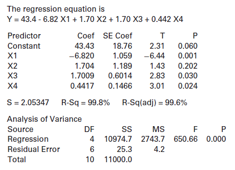
What is the coefficient of X1 in the model? What is the p-value for testing this coefficient?Refer to the multiple regression output shown: The regression equation is Y = 43.4 - 6.82 X1 + 1.70 X2 + 1.70 X3 + 0.442 X4 Predictor Coef SE Coef т Constant 43.43 18.76 2.31 0.060 1.059 X1 -6.820 -6.44
Use the information that, for events A and B, we have P(A) = 0.4, P(B) = 0. Find P(not B)..3, and P(A and B) = 0.1.Find P(not A).
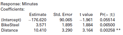
Distance is associated with both the type of bike and commute time, so if we are really interested in which type of bike is faster, we should account for the confounding variable Distance. Output regressing Minutes on both BikeSteel and Distance (measured in miles) is shown below.Residual standard
Which of the variables are significant at the 5% level?Refer to the multiple regression output shown: The regression equation is Y = 43.4 - 6.82 X1 + 1.70 X2 + 1.70 X3 + 0.442 X4 Predictor Coef SE Coef т Constant 43.43 18.76 2.31 0.060 1.059 X1 -6.820 -6.44 0.001 X2 1.704 1.189 1.43 0.202 2.83
Which of the variables are significant at the 1% level?Refer to the multiple regression output shown: The regression equation is Y = 43.4 - 6.82 X1 + 1.70 X2 + 1.70 X3 + 0.442 X4 Predictor Coef SE Coef т Constant 43.43 18.76 2.31 0.060 1.059 X1 -6.820 -6.44 0.001 X2 1.704 1.189 1.43 0.202 2.83
What is the coefficient of X2 in the model? What is the p-value for testing this coefficient?Refer to the multiple regression output shown: The regression equation is Y = 43.4 - 6.82 X1 + 1.70 X2 + 1.70 X3 + 0.442 X4 Predictor Coef SE Coef т Constant 43.43 18.76 2.31 0.060 1.059 X1 -6.820 -6.44
One case in the sample has Y = 60, X1 = 5, X2 = 7, X3 = 5, and X4 = 75. What is the predicted response for this case? What is the residual?Refer to the multiple regression output shown: The regression equation is Y = 43.4 - 6.82 X1 + 1.70 X2 + 1.70 X3 + 0.442 X4 Predictor Coef SE Coef т Constant
One case in the sample has Y = 30, X1 = 8, X2 = 6,X3 = 4, andX4 = 50. What is the predicted response for this case? What is the residual?Refer to the multiple regression output shown: The regression equation is Y = 43.4 - 6.82 X1 + 1.70 X2 + 1.70 X3 + 0.442 X4 Predictor Coef SE Coef т Constant
What are the explanatory variables? What is the response variable?Refer to the multiple regression output shown: The regression equation is Y = 43.4 - 6.82 X1 + 1.70 X2 + 1.70 X3 + 0.442 X4 Predictor Coef SE Coef т Constant 43.43 18.76 2.31 0.060 1.059 X1 -6.820 -6.44 0.001 X2 1.704 1.189 1.43
Which variable is most significant in this model?Refer to the multiple regression output shown: The regression equation is Y = 43.4 - 6.82 X1 + 1.70 X2 + 1.70 X3 + 0.442 X4 Predictor Coef SE Coef т Constant 43.43 18.76 2.31 0.060 1.059 X1 -6.820 -6.44 0.001 X2 1.704 1.189 1.43 0.202 2.83 ХЗ
Which variable is least significant in this model?Refer to the multiple regression output shown: The regression equation is Y = 43.4 - 6.82 X1 + 1.70 X2 + 1.70 X3 + 0.442 X4 Predictor Coef SE Coef т Constant 43.43 18.76 2.31 0.060 1.059 X1 -6.820 -6.44 0.001 X2 1.704 1.189 1.43 0.202 2.83 ХЗ
Is the model effective, according to the ANOVA test? Justify your answer.Refer to the multiple regression output shown: The regression equation is Y = 43.4 - 6.82 X1 + 1.70 X2 + 1.70 X3 + 0.442 X4 Predictor Coef SE Coef т Constant 43.43 18.76 2.31 0.060 1.059 X1 -6.820 -6.44 0.001 X2 1.704 1.189
State and interpret R2for this model.Refer to the multiple regression output shown: The regression equation is Y = 43.4 - 6.82 X1 + 1.70 X2 + 1.70 X3 + 0.442 X4 Predictor Coef SE Coef т Constant 43.43 18.76 2.31 0.060 1.059 X1 -6.820 -6.44 0.001 X2 1.704 1.189 1.43 0.202 2.83 ХЗ 1.7009 0.6014
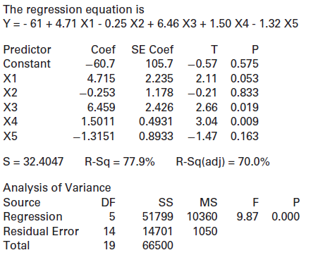
One case in the sample has Y = 20, X1 = 15, X2 = 40, X3 = 10, X4 = 50, and X5 = 95. What is the predicted response for this case? What is the residual?Refer to the multiple regression output shown: The regression equation is Y = - 61 + 4.71 X1 - 0.25 X2 + 6.46 X3 + 1.50 X4 - 1.32 X5 Predictor Coef
One case in the sample has Y = 50, X1 = 19, X2 = 56, X3 = 12, X4 = 85, and X5 = 106. What is the predicted response for this case? What is the residual?Refer to the multiple regression output shown: The regression equation is Y = - 61 + 4.71 X1 - 0.25 X2 + 6.46 X3 + 1.50 X4 - 1.32 X5 Predictor Coef
What is the coefficient of X1 in the model? What is the p-value for testing this coefficient?Refer to the multiple regression output shown: The regression equation is Y = - 61 + 4.71 X1 - 0.25 X2 + 6.46 X3 + 1.50 X4 - 1.32 X5 Predictor Coef SE Coef т Constant -60.7 105.7 -0.57 0.575 X1 4.715 2.235
What is the coefficient of X5 in the model? What is the p-value for testing this coefficient?Refer to the multiple regression output shown: The regression equation is Y = - 61 + 4.71 X1 - 0.25 X2 + 6.46 X3 + 1.50 X4 - 1.32 X5 Predictor Coef SE Coef т Constant -60.7 105.7 -0.57 0.575 X1 4.715 2.235
Which of the variables are significant at the 5% level?Refer to the multiple regression output shown: The regression equation is Y = - 61 + 4.71 X1 - 0.25 X2 + 6.46 X3 + 1.50 X4 - 1.32 X5 Predictor Coef SE Coef т Constant -60.7 105.7 -0.57 0.575 X1 4.715 2.235 2.11 0.053 X2 -0.253 1.178 -0.21
Which of the variables are significant at the 1% level?Refer to the multiple regression output shown: The regression equation is Y = - 61 + 4.71 X1 - 0.25 X2 + 6.46 X3 + 1.50 X4 - 1.32 X5 Predictor Coef SE Coef т Constant -60.7 105.7 -0.57 0.575 X1 4.715 2.235 2.11 0.053 X2 -0.253 1.178 -0.21
Which variable is most significant in this model?Refer to the multiple regression output shown: The regression equation is Y = - 61 + 4.71 X1 - 0.25 X2 + 6.46 X3 + 1.50 X4 - 1.32 X5 Predictor Coef SE Coef т Constant -60.7 105.7 -0.57 0.575 X1 4.715 2.235 2.11 0.053 X2 -0.253 1.178 -0.21 0.833 XЗ
Which variable is least significant in this model?Refer to the multiple regression output shown: The regression equation is Y = - 61 + 4.71 X1 - 0.25 X2 + 6.46 X3 + 1.50 X4 - 1.32 X5 Predictor Coef SE Coef т Constant -60.7 105.7 -0.57 0.575 X1 4.715 2.235 2.11 0.053 X2 -0.253 1.178 -0.21 0.833 XЗ
Is the model effective, according to the ANOVA test? Justify your answer.Refer to the multiple regression output shown: The regression equation is Y = - 61 + 4.71 X1 - 0.25 X2 + 6.46 X3 + 1.50 X4 - 1.32 X5 Predictor Coef SE Coef т Constant -60.7 105.7 -0.57 0.575 X1 4.715 2.235 2.11 0.053 X2
State and interpret R2for this model.Refer to the multiple regression output shown: The regression equation is Y = - 61 + 4.71 X1 - 0.25 X2 + 6.46 X3 + 1.50 X4 - 1.32 X5 Predictor Coef SE Coef т Constant -60.7 105.7 -0.57 0.575 X1 4.715 2.235 2.11 0.053 X2 -0.253 1.178 -0.21 0.833 XЗ 6.459 2.426
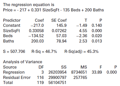
Here is some output for fitting a model to predict the price of a home (in $1000s) using size (in square feet, SizeSqFt, different units than the variable Size in HomesForSale), number of bedrooms, and number of bathrooms. (The data are based indirectly on information in the HomesForSale
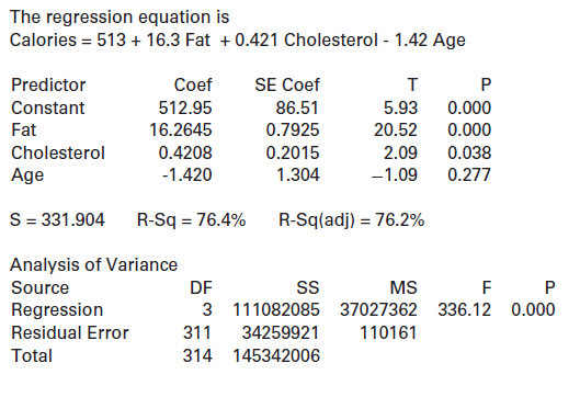
Using the data in NutritionStudy, we show computer output for a model to predict calories consumed in a day based on fat grams consumed in a day, cholesterol consumed in mg per day, and age in years:(a) What daily calorie consumption does the model predict for a 35 year old person who eats 40 grams
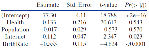
In Exercises 9.25 and 9.64 we attempt to predict a country€™s life expectancy based on the percent of government expenditure on health care, using a sample of fifty countries in the dataset SampCountries. We now add to the model the variables population (in millions), percentage with
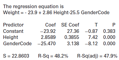
Categorical variables with only two categories (such as male/female or yes/no) can be used in a multiple regression model if we code the answers with numbers. In Chapter 9, we looked at a simple linear model to predict Weight based on Height. What role does gender play? If a male and a female are
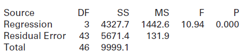
How many predictors are in the model?Use information in the ANOVA table below, which comes from fitting a multiple regression model to predict the prices for horses (in $1000s). Source Regression Residual Error Total DF SS MS 4327.7 5671.4 1442.6 131.9 10.94 0.000 43 46 9999.1
How many horses are in the sample?Use information in the ANOVA table below, which comes from fitting a multiple regression model to predict the prices for horses (in $1000s). Source Regression Residual Error Total DF SS MS 4327.7 5671.4 1442.6 131.9 10.94 0.000 43 46 9999.1
Find and interpret (as best you can with the given context) the value of R2.Use information in the ANOVA table below, which comes from fitting a multiple regression model to predict the prices for horses (in $1000s). Source Regression Residual Error Total DF SS MS 4327.7 5671.4 1442.6 131.9 10.94
Is this an effective model for predicting horse prices? Write down the relevant hypotheses as well as a conclusion based on the ANOVA table.Use information in the ANOVA table below, which comes from fitting a multiple regression model to predict the prices for horses (in $1000s). Source Regression
In Exercise 9.23 on page 537, we discuss a study conducted on the California Channel Islands investigating the prevalence of hantavirus in mice. This virus can cause severe lung disease in humans. The article states: ‘‘Precipitation accounted for 79% of the variation in prevalence. Adding in
In Exercise 9.63 we look at predicting the price (in $1000s) of New York homes based on the size (in thousands of square feet), using the data in HomesForSaleNY. Two other variables in the dataset are the number of bedrooms and the number of bathrooms. Use technology to create a multiple regression
Use technology and the data in LightatNight to predict body mass gain in mice, BMGain, over a fourweek experiment based on stress levels measured in Corticosterone, percent of calories eaten during the day (most mice in the wild eat all calories at night) DayPct, average daily consumption of food
In Exercise 9.26 on page 538 we consider simple linear models to predict winning percentages for NBA teams based on either their offensive ability (PtsFor = average points scored per game) or defensive ability (PtsAgainst = average points allowed per game). With multiple regression we can include
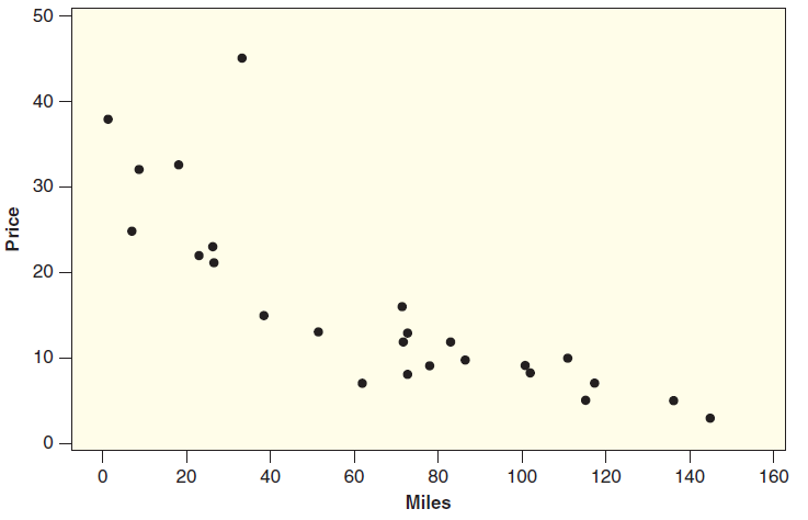
Data 3.4 on page 209 describes a sample of n = 25 Mustang cars being offered for sale on the Internet. We would like to predict the Price of used Mustangs (in $1000s) and the possible explanatory variables in MustangPrice are the Age in years and Miles driven (in 1000s).(a) Fit a simple linear
In Exercise 9.26 on page 538 we consider separate simple linear models to predict NBA winning percentages using PtsFor and PtsAgainst. In Exercise 10.34 we combine these to form a multiple regression model. The data is in NBAStandings.(a) Compare the percentages of variability in winning
When deriving the F-statistic on page 541 we include a note that the use of the F-distribution can be simulated with a randomization procedure. That is the purpose of this exercise. Consider the model in Example 10.7 that uses PhotoTime and CostColor to predict inkjet printer prices. The
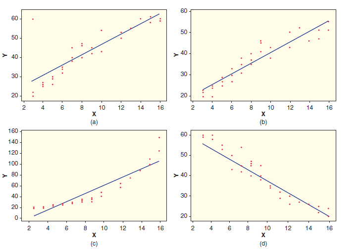
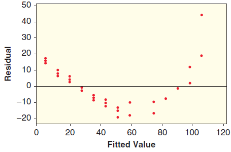
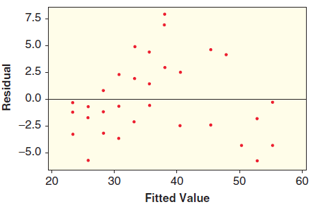
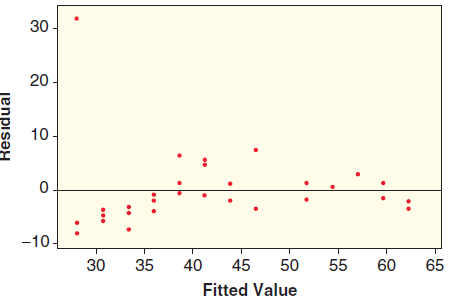
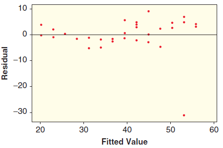
Give scatterplots of residuals against predicted values. Match each with one of the scatterplots shown in Figure 10.7. 60 - 60 - 50 > 40. > 40- 30 30 : 20 20 8. 10 12 14 16 4 6. 8. 10 12 14 16 (a) (b) 160 60 140 120 50 100 - > 80 > 40 60 30 40 20 - 20 8. 10 12 14 16 6. 8. 10 12 14 16 (c) (d) .co 2.
Give scatterplots of residuals against predicted values. Match each with one of the scatterplots shown in Figure 10.7. 60 - 60 - 50 > 40. > 40- 30 30 : 20 20 8. 10 12 14 16 4 6. 8. 10 12 14 16 (a) (b) 160 60 140 120 50 100 - > 80 > 40 60 30 40 20 - 20 8. 10 12 14 16 6. 8. 10 12 14 16 (c) (d) .co 2.
Give scatterplots of residuals against predicted values. Match each with one of the scatterplots shown in Figure 10.7. 60 - 60 - 50 > 40. > 40- 30 30 : 20 20 8. 10 12 14 16 4 6. 8. 10 12 14 16 (a) (b) 160 60 140 120 50 100 - > 80 > 40 60 30 40 20 - 20 8. 10 12 14 16 6. 8. 10 12 14 16 (c) (d) .co 2.
Give scatterplots of residuals against predicted values. Match each with one of the scatterplots shown in Figure 10.7. 60 - 60 - 50 > 40. > 40- 30 30 : 20 20 8. 10 12 14 16 4 6. 8. 10 12 14 16 (a) (b) 160 60 140 120 50 100 - > 80 > 40 60 30 40 20 - 20 8. 10 12 14 16 6. 8. 10 12 14 16 (c) (d) .co 2.
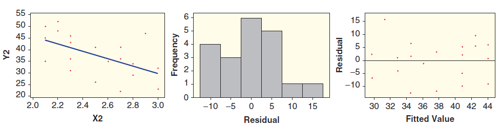
Three graphs are shown for a linear model: the scatterplot with least squares line, a histogram of the residuals, and a scatterplot of residuals against predicted values. Determine whether the conditions are met and explain your reasoning. 55 15 50 45 10 40 35 30 25 -5 -10 20 2.2 2.0 2.6 2.8 10 15
Using the data in StudentSurvey, we see that the regression line to predict Weight from Height isFigure 10.8 shows three graphs for this linear model: the scatterplot with least squares line, a histogram of the residuals, and a scatterplot of residuals against predicted values.Figure 10.8(a) One of
As we see in Exercise 10.44, or by using the data in StudentSurvey, the regression line to predict Weight from Height isFigure 10.8 shows three graphs for this linear model: the scatterplot with least squares line, a histogram of the residuals, and a scatterplot of residuals against predicted
Use the data in StudentSurvey to assess the conditions for doing inference on a regression model to predict a person’s pulse rate, Pulse, from the number of hours a week spent exercising, Exercise. Explain your reasoning, using each of the three relevant graphs.Data in StudentSurveyData on 362
Use the data in NutritionStudy to assess the conditions for doing inference on a regression model to predict a person’s daily calories, Calories, from the daily grams of fat, Fat. Explain your reasoning, using each of the three relevant graphs.Data in NutritionStudy Data on 315 patients
Use the data in NutritionStudy to assess the conditions for doing inference on a regression model to predict a person’s cholesterol level, Cholesterol, from the daily grams of fat, Fat. Explain your reasoning, using each of the three relevant graphs.Data in NutritionStudy Data on 315
Use the data in RestaurantTips to assess the conditions for doing inference on a regression line to predict the size of a customer’s tip, Tip, from the size of the bill, Bill. Explain your reasoning, using each of the three relevant graphs.Data in RestaurantTipsThe owner of a bistro called First
The data in CommuteAtlanta show information on both the commute distance (in miles) and time (in minutes) for a sample of 500 Atlanta commuters. Suppose that we want to build a model for predicting the commute time based on the distance.(a) Fit the simple linear model, Time = β0 +
Refer to Exercise 10.50. The file CommuteStLouis contains similar information for a sample of 500 commuters in St. Louis. Answer the same questions as Exercise 10.50 using the St. Louis data. Are the results in St. Louis much different from Atlanta?Exercise 10.50The data in CommuteAtlanta show
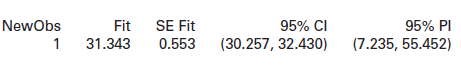
In Exercise 10.50 we consider a simple linear model to predict Time in minutes for Atlanta commuters based on Distance in miles using the data in CommuteAtlanta. For a 20 mile commute the predicted time is 31.34 minutes. Here is some output containing intervals for this prediction.(a) Interpret the
In Exercise 10.32 on page 571, we use the data in HomesForSaleNY to predict prices for houses based on size, number of bedrooms, and number of bathrooms. Use technology to find the residuals for fitting that model and construct appropriate residual plots to assess whether the conditions for a
In Exercise 10.33 on page 571, we use the data in LightatNight to predict body mass gain in mice (BMGain) over a four-week experiment based on stress levels measured in Corticosterone, percent of calories eaten during the day (most mice in the wild eat all calories at night) DayPct, average daily
In Exercise 10.34 on page 571, we use the data in NBAStandings to predict NBA winning percentage based on PtsFor and PtsAgainst. Use technology to find the residuals for fitting that model and construct appropriate residual plots to assess whether the conditions for a multiple regression model are
In Exercise 10.35 on page 571, we use the data in MustangPrice to predict the Price of used Mustang cars based on the Age in years and number of Miles driven. Use technology to find the residuals for fitting that model and construct appropriate residual plots to assess whether the conditions for a
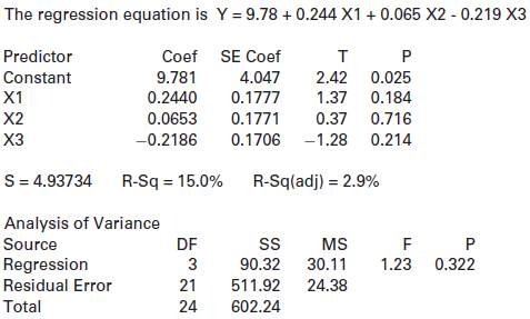
Use the multiple regression output shown to answer the following questions.(a) Which variable might we try eliminating first to possibly improve this model?(b) What is R2 for this model? Do we expect R2 to increase, decrease, or remain the same if we eliminate the variable chosen in part (a)? What
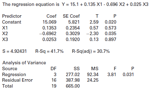
Use the multiple regression output shown to answer the following questions.(a) Which variable might we try eliminating first to possibly improve this model?(b) What is R2 for this model? Do we expect R2 to increase, decrease, or remain the same if we eliminate the variable chosen in part (a)? What
The dataset HollywoodMovies2011 includes information on movies that came out of Hollywood in 2011. We want to build a model to predict Profitability, which is the percent of the budget recovered in profits. Start with a model including the following five explanatory variables:RottenTomatoes
The dataset FloridaLakes includes information on lake water in Florida. We want to build a model to predict AvgMercury, which is the average mercury level of fish in the lake. Start with a model including the following four explanatory variables: Alkalinity, pH, Calcium, and Chlorophyll. Eliminate
Baseball is played at a fairly leisurely pace—in fact, sometimes too slow for some sports fans. What contributes to the length of a major league baseball game? The file BaseballTimes contains information from a sample of 30 games to help build a model for the time of a game (in minutes).
Use the data in AllCountries to answer the following questions.(a) Is electricity use a significant single predictor of life expectancy?(b) Explain why GDP (per-capita Gross Domestic Product) is a potential confounding variable in the relationship between Electricity and LifeExpectancy.(c) Is
Use the data in AllCountries to answer the following questions.(a) Is the number of mobile subscriptions per 100 people, Cell, a significant single predictor of life expectancy?(b) Explain why GDP (per-capita Gross Domestic Product) is a potential confounding variable in the relationship between
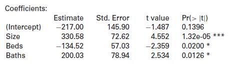
In Exercise 10.23 on page 569 we fit a model predicting the price of a home (in $1000s), using size (in square feet), number of bedrooms, and number of bathrooms, based on data in HomesForSale. Output for fitting a slightly revised model is shown below where the Size variable is measured in 1000s
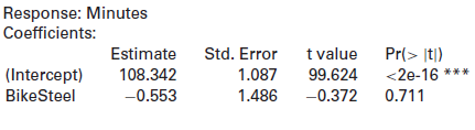
Output regressing Minutes on BikeSteel is shown below.Residual standard error: 5.545 on 54 degrees of freedomMultiple R-squared: 0.002558, Adjusted R-squared: -0.01591F-statistic: 0.1385 on 1 and 54 DF, p-value: 0.7112(a) What is Dr. Grove€™s predicted commute time if riding the steel
In Exercise 10.66, regressing Minutes on BikeSteel, the coefficient for BikeSteel is negative. In Exercise 10.68, regressing Minutes on BikeSteel and Distance, the coefficient for BikeSteel is positive.(a) A biker interested in whether carbon or steel bikes are faster is not sure what to make of
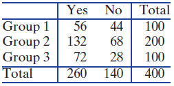
Refer to the table below. In each case, give the degrees of freedom for the chi-square test based on that two-way table.Two-way table in Exercise 7.31(Group 3, Yes) cell Yes No Total 56 44 Group 1 Group 2 132 Group 3 72 260 100 68 200 28 100 140 Total 400
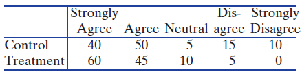
Refer to the table below. In each case, give the degrees of freedom for the chi-square test based on that two-way table.Two-way table in Exercise 7.32(Control, Disagree) cell Dis- Strongly Agree Agree Neutral agree Disagree 10 Strongly Control Treatment 40 15 50 45 5 10 60
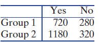
Refer to the table below. In each case, give the degrees of freedom for the chi-square test based on that two-way table.Two-way table in Exercise 7.33(Group 2, No) cell No 720 280 Group 2| 1180 320 Yes Group 1
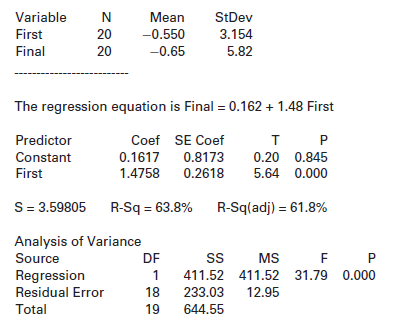
In a professional golf tournament the players participate in four rounds of golf and the player with the lowest score after all four rounds is the champion. How well does a player€™s performance in the first round of the tournament predict the final score? Table 9.6 shows the first round
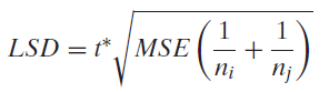
One way to €˜€˜automate€ pairwise comparisons that works particularly well when the sample sizes are balanced is to compute a single value that can serve as a threshold for when a pair of sample means are far enough apart to suggest that the population means differ $LSD = t*,| MSE \Ni пj$
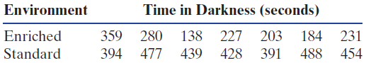
Use Fisher€™s LSD, as described in Exercise 8.50, to discuss differences in mean time mice spend in darkness for the six combinations of environment and stress that produce the output in Exercise 8.49.Exercise 8.49Many studies have shown that people who engage in any exercise have $LSD = t*,| MSE \Ni пj$
In Exercise 8.32 on page 512 we consider an ANOVA to test for difference in mean gill beat rates for fish in water with three different levels of calcium. The data are stored in FishGills3. If the ANOVA table indicates that the mean gill rates differ due to the calcium levels, determine which
The dataset HomesForSaleCA contains a random sample of 30 houses for sale in California. We are interested in whether there is a positive association between the number of bathrooms and number of bedrooms in each house.(a) What are the null and alternative hypotheses for testing the correlation?(b)
A random sample of 50 countries is stored in the dataset SampCountries. Two variables in the dataset are life expectancy (LifeExpectancy) and percentage of government expenditure spent on health care (Health) for each country.Weare interested in whether or not the percent spent on health care can
A common (and hotly debated) saying among sports fans is ‘‘Defense wins championships.’’ Is offensive scoring ability or defensive stinginess a better indicator of a team’s success? To investigate this question we’ll use data from the 2010–11 National Basketball Association (NBA)
Use the dataset AllCountries to examine the correlation between birth rate and life expectancy across countries of the world.(a) Plot the data. Do birth rate and life expectancy appear to be linearly associated?(b) From this dataset, can we conclude that the population correlation between birth
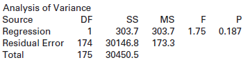
We show an ANOVA table for regression. State the hypotheses of the test, give the F-statistic and the p-value, and state the conclusion of the test. Analysis of Variance Source Regression Residual Error 174 Total MS 303.7 1.75 0.187 173.3 DF 303.7 30146.8 175 30450.5
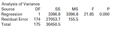
We show anANOVAtable for regression. State the hypotheses of the test, give the F-statistic and the p-value, and state the conclusion of the test. Analysis of Variance Source Regression Residual Error 174 Total DF 3396.8 3396.8 21.85 0.000 27053.7 MS 155.5 30450.5 175
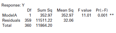
We show anANOVAtable for regression. State the hypotheses of the test, give the F-statistic and the p-value, and state the conclusion of the test. Response: Y Df Sum Sq Mean Sq Fvalue Pr(>F) 11.01 0.001 ** 352.97 352.97 32.06 1 ModelA Residuals 359 11511.22 Total 360 11864.20
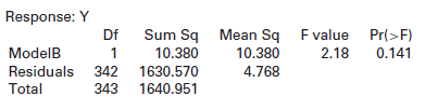
We show anANOVAtable for regression. State the hypotheses of the test, give the F-statistic and the p-value, and state the conclusion of the test. Response: Y Sum Sq Mean Sq Fvalue Pr(>F) Df ModelB Residuals 342 10.380 1630.570 1640.951 10.380 4.768 2.18 0.141 Total 343

Showing 400 - 500 of 2108

1
2
3
4
5
6
7
8
9
10
11
12
13
14
15
Last

Step by Step Answers

Services

Sitemap
Fun
Definitions
Become Tutor
Used Textbooks
Study Help Categories
Recent Questions
Expert Questions
Campus Wear
Sell Your Books

Company Info

Security
Copyrights
Privacy Policy
Terms & Conditions
SolutionInn Fee
Scholarship
Online Quiz
Give Feedback, Get Rewards

Get In Touch

About Us
Contact Us
Career
Jobs
FAQ
Student Discount
Campus Ambassador

Secure Payment

Download Our App

© 2026 SolutionInn. All Rights Reserved