New Semester
Started
Get
50% OFF
Study Help!
--h --m --s
Claim Now
Question Answers
Textbooks
Find textbooks, questions and answers
Oops, something went wrong!
Change your search query and then try again
S
Books
FREE
Study Help
Expert Questions
Accounting
General Management
Mathematics
Finance
Organizational Behaviour
Law
Physics
Operating System
Management Leadership
Sociology
Programming
Marketing
Database
Computer Network
Economics
Textbooks Solutions
Accounting
Managerial Accounting
Management Leadership
Cost Accounting
Statistics
Business Law
Corporate Finance
Finance
Economics
Auditing
Tutors
Online Tutors
Find a Tutor
Hire a Tutor
Become a Tutor
AI Tutor
AI Study Planner
NEW
Sell Books
Search
Search
Sign In
Register
study help
mathematics
statistics the art and science
Statistics Unlocking The Power Of Data 1st Edition Robin H. Lock, Patti Frazer Lock, Kari Lock Morgan, Eric F. Lock, Dennis F. Lock - Solutions
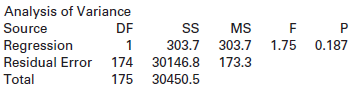
Use the information in the table to give the sample size and to calculate R2.The ANOVA table in Exercise 9.28 Analysis of Variance Source Regression Residual Error 174 Total MS 303.7 1.75 0.187 173.3 DF 303.7 30146.8 175 30450.5
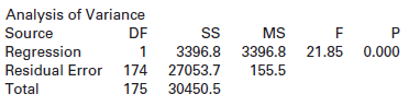
Use the information in the table to give the sample size and to calculate R2.The ANOVA table in Exercise 9.29 Analysis of Variance Source Regression Residual Error 174 Total DF 3396.8 3396.8 21.85 0.000 27053.7 MS 155.5 30450.5 175
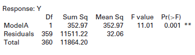
Use the information in the table to give the sample size and to calculate R2.The ANOVA table in Exercise 9.30 Response: Y Df Sum Sq Mean Sq Fvalue Pr(>F) 11.01 0.001 ** 352.97 352.97 32.06 1 ModelA Residuals 359 11511.22 Total 360 11864.20
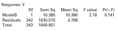
Use the information in the table to give the sample size and to calculate R2.The ANOVA table in Exercise 9.31 Response: Y Sum Sq Mean Sq Fvalue Pr(>F) Df ModelB Residuals 342 10.380 1630.570 1640.951 10.380 4.768 2.18 0.141 Total 343
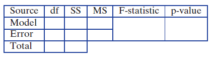
SSModel = 250 with SSTotal = 3000 and a sample size of n = 100We give some information about sums of squares and sample size for a linear model. Use this information to fill in all values in an analysis of variance for regression table as shown. df SS F-statistic | p-value Source Model MS Error
SSModel = 800 with SSTotal = 5820 and a sample size of n = 40We give some information about sums of squares and sample size for a linear model. Use this information to fill in all values in an analysis of variance for regression table as shown. df SS F-statistic | p-value Source Model MS Error Total
SSModel = 8.5 with SSError = 247.2 and a sample size of n = 25We give some information about sums of squares and sample size for a linear model. Use this information to fill in all values in an analysis of variance for regression table as shown. df SS F-statistic | p-value Source Model MS Error
SSError = 15,571 with SSTotal = 23,693 and a sample size of n = 500We give some information about sums of squares and sample size for a linear model. Use this information to fill in all values in an analysis of variance for regression table as shown. df SS F-statistic | p-value Source Model MS
Exercise 9.19 on page 536 introduces a study examining the relationship between the number of friends an individual has on Facebook and grey matter density in the areas of the brain associated with social perception and associative memory. The data are available in the dataset FacebookFriends and
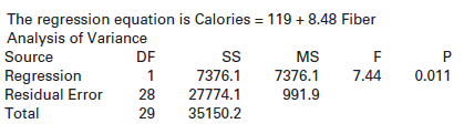
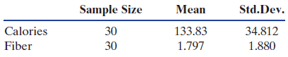
In Data 9.2 on page 540, we introduce the dataset Cereal, which has nutrition information on 30 breakfast cereals. Computer output is shown for a linear model to predict Calories in one cup of cereal based on the number of grams of Fiber. Is the linear model effective at predicting the number of
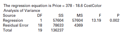
Data 9.1 on page 525 introduces the dataset InkjetPrinters, which includes information on all-in-one printers. Two of the variables are Price (the price of the printer in dollars) and CostColor (average cost per page in cents for printing in color). Computer output for predicting the price from the
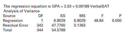
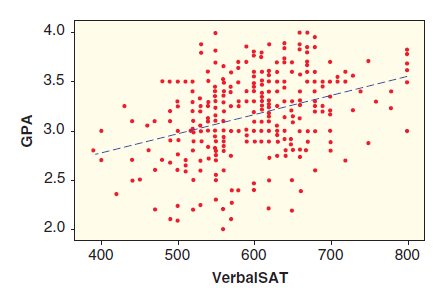
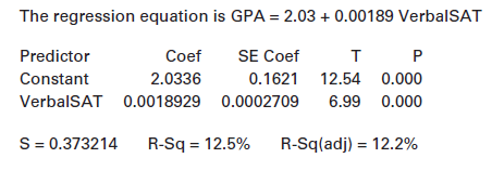
How well does a student€™s Verbal SAT score (on an 800-point scale) predict future college grade point average (on a four-point scale)? Computer output for this regression analysis is shown, using the data in StudentSurvey:(a) What is the predicted grade point average of a student who
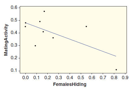
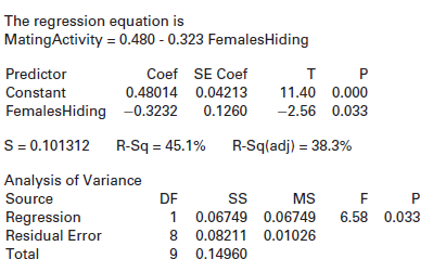
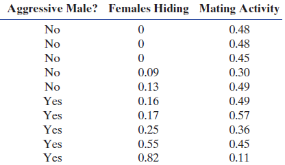
In Exercise A.46 on page 153, we introduce a study about mating activity of water striders. The dataset is available as WaterStriders and includes the variables FemalesHiding, which gives the proportion of time the female water striders were in hiding, and MatingActivity, which is a measure of mean
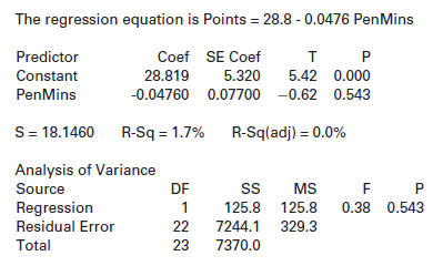
The dataset OttawaSenators contains information on the number of points and the number of penalty minutes for 24 Ottawa Senators NHL hockey players. Computer output is shown for predicting the number of points from the number of penalty minutes:(a) Write down the equation of the least squares line
Exercise 9.41 gives output for a regression model to predict calories in a serving of breakfast cereal based on the number of grams of fiber in the serving. Use this output, together with any helpful summary statistics from Table 9.3, to show how to calculate the following regression
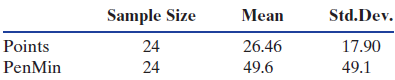
Exercise 9.45 gives output for a regression model to predict number of points for a hockey player based on the number of penalty minutes for the hockey player. Use this output, together with any helpful summary statistics from Table 9.2, to show how to calculate the regression quantities given in
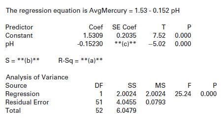
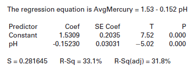
In Exercise 9.21, we see that the conditions are met for using the pH of a lake in Florida to predict the mercury level of fish in the lake. The data are given in FloridaLakes. Computer output is shown for the linear model with several values missing:(a) Use the information in the ANOVA table to
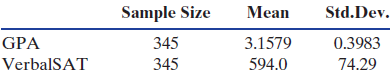
Exercise 9.43 gives output for a regression model to predict grade point average in college based on score on the Verbal SAT exam. Use this output, together with any helpful summary statistics from Table 9.4, to calculate the following regression quantities:Table 9.4(a) The standard deviation of
Consider a simple linear model for the number of hours of exercise students get (per week) based on the number of hours spent watching TV. Use the data in ExerciseHours to fit this model. Test the effectiveness of the TV predictor three different ways as requested below, giving hypotheses, test
In Exercise 9.25 we see that the conditions are met for fitting a linear model to predict life expectancy (LifeExpectancy) from the percentage of government expenditure spent on health care (Health) using the data in SampCountries. Use technology to examine this relationship further, as requested
The dataset HomesForSaleCA contains a random sample of 30 houses for sale in California. We are interested in whether we can use number of bathrooms Baths to predict number of bedrooms Beds in houses in California. Use technology to answer the following questions:(a) What is the fitted regression
Consider the data described in Exercise 9.52 on homes for sale in California and suppose that we are interested in predicting the Size (in thousands of square feet) for such homes.(a) What is the total variability in the sizes of the 30 homes in this sample? ANOVA with any of the other variables as
Two intervals are given, A and B, for the same value of the explanatory variable. In each case:(a) Which interval is the confidence interval for the mean response? Which interval is the prediction interval for the response?(b) What is the predicted value of the response variable for this value of
Two intervals are given, A and B, for the same value of the explanatory variable. In each case:(a) Which interval is the confidence interval for the mean response? Which interval is the prediction interval for the response?(b) What is the predicted value of the response variable for this value of
Two intervals are given, A and B, for the same value of the explanatory variable. In each case:(a) Which interval is the confidence interval for the mean response? Which interval is the prediction interval for the response?(b) What is the predicted value of the response variable for this value of
Two intervals are given, A and B, for the same value of the explanatory variable. In each case:(a) Which interval is the confidence interval for the mean response? Which interval is the prediction interval for the response?(b) What is the predicted value of the response variable for this value of
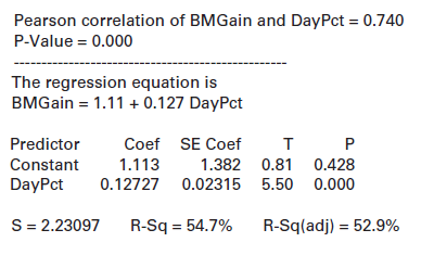
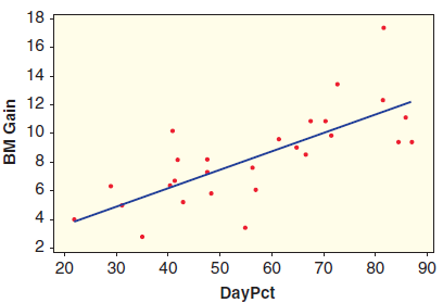
The intervals given are for mice that eat 50% of their calories during the day:In Exercise 9.18 on page 535, we look at a model to predict weight gain (in grams) in mice based on the percent of calories the mice eat during the day (when mice should be sleeping instead of eating). We give computer
The intervals given are for mice that eat 10% of their calories during the day:In Exercise 9.18 on page 535, we look at a model to predict weight gain (in grams) in mice based on the percent of calories the mice eat during the day (when mice should be sleeping instead of eating). We give computer
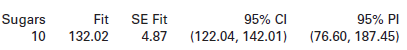
The intervals given are for cereals with 10 grams of sugars:In Example 9.10 on page 540, we look at a model to predict the number of calories in a cup of breakfast cereal using the number of grams of sugars. We give computer output with two regression intervals and information about a specific
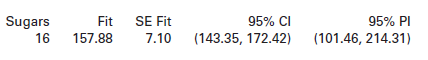
The intervals given are for cereals with 16 grams of sugars:In Example 9.10 on page 540, we look at a model to predict the number of calories in a cup of breakfast cereal using the number of grams of sugars. We give computer output with two regression intervals and information about a specific
People in real estate are interested in predicting the price of a house by the square footage, and predictions will vary based on geographic area. We look at predicting prices (in $1000s) of houses in New York state based on the size (in thousands of square feet). A random sample of 30 houses for
In Exercise 9.25 on page 555, we consider a regression equation to predict life expectancy from percent of government expenditure on health care, using data for a sample of 50 countries in SampCountries. Using technology and this dataset, find and interpret a 95% prediction interval for each of the
Exercise 9.17 on page 535, we use the information in StudentSurvey to fit a linear model to use Verbal SAT score to predict a student€™s grade point average in college. The regression equation is(a) What GPA does the model predict for a student who gets a 500 on the Verbal SAT exam? What
Data 2.9 on page 103 introduces data on the approval rating of an incumbent US president and the margin of victory or defeat in the subsequent election (where negative numbers indicate the margin by which the incumbent president lost the re-election campaign). The data are reproduced in Table 9.5
Hantavirus is carried by wild rodents and causes severe lung disease in humans. A recent study on the California Channel Islands found that increased prevalence of the virus was linked with greater precipitation. The study adds ‘‘Precipitation accounted for 79% of the variation in
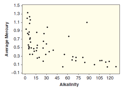
The FloridaLakes dataset, introduced in Data 2.4, includes data on 53 lakes in Florida. Figure 9.10 shows a scatterplot of Alkalinity (concentration of calcium carbonate in mg/L) and AvgMercury (average mercury level for a sample of fish from each lake). Explain using the conditions for a linear
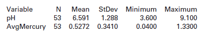
The FloridaLakes dataset, introduced in Data 2.4, includes data on 53 lakes in Florida. Two of the variables recorded are pH (acidity of the lake water) and AvgMercury (average mercury level for a sample of fish from each lake). We wish to use the pH of the lake water (which is easy to measure) to
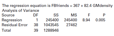
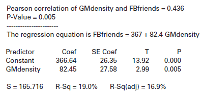
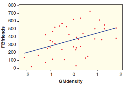
In Exercise 9.19, we give computer output for a regression line to predict the number of Facebook friends a student will have, based on a normalized score of the grey matter density in the areas of the brain associated with social perception and associative memory. Data for the sample of n = 40
A recent study in Great Britain examines the relationship between the number of friends an individual has on Facebook and grey matter density in the areas of the brain associated with social perception and associative memory. The data are available in the dataset FacebookFriends and the relevant
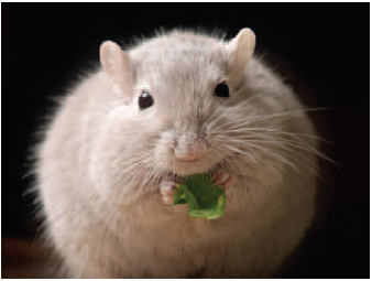
Data A.1 on page 136 introduces a study that examines the effect of light at night on weight gain in a sample of 27 mice observed over a fourweek period. The mice who had a light on at night gained significantly more weight than the mice with darkness at night, despite eating the same number of
A scatterplot with regression line is shown in Figure 9.7 for a regression model using Verbal SAT score, VerbalSAT, to predict grade point average in college, GPA, using the data in StudentSurvey. We also show computer output below of the regression analysis.Figure 9.7(a) Use the scatterplot to
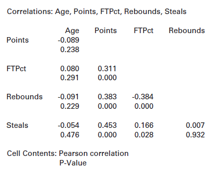
The dataset NBAPlayers2011 is introduced on page 88 and contains information on many variables for players in the NBA (National Basketball Association) during the 2010€“11 season. The dataset includes information for all players who averaged more than 24 minutes per game (n = 176) and 24
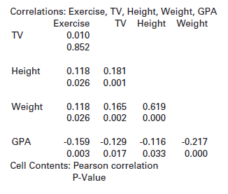
A correlation matrix allows us to see lots of correlations at once, between many pairs of variables.Acorrelation matrix for several variables (Exercise, TV, Height, Weight, and GPA) in the StudentSurvey dataset is given. For any pair of variables (indicated by the row and the column), we are given
Test for a negative correlation; r = −0.41; n = 18Test the correlation, as indicated. Show all details of the test.
Test for evidence of a linear association; r = 0.28; n = 100Test the correlation, as indicated. Show all details of the test.
Test for evidence of a linear association; r = 0.28; n = 10Test the correlation, as indicated. Show all details of the test.
Test for a positive correlation; r = 0.35; n = 30Test the correlation, as indicated. Show all details of the test.
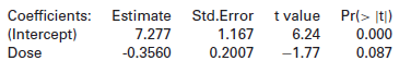
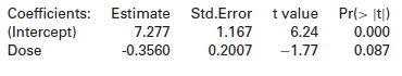
The model given by the output in Exercise 9.7, with n = 30.Exercise 9.7Find and interpret a 95% confidence interval for the slope of the model indicated. Coefficients: Estimate Std.Error t value Pr(> [t]) 1.167 7.277 | (Intercept) Dose 6.24 -1.77 0.000 0.087 -0.3560 0.2007
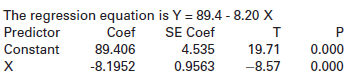
The model given by the output in Exercise 9.5, with n = 24.Exercise 9.5Find and interpret a 95% confidence interval for the slope of the model indicated. The regression equation is Y = 89.4 - 8.20 X SE Coef 4.535 0.9563 Predictor Constant Coef 89.406 -8.1952 т 19.71 -8.57 0.000 0.000
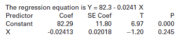
Show some computer output for fitting simple linear models. State the value of the sample slope for each model and give the null and alternative hypotheses for testing if the slope in the population is different from zero. Identify the p-value and use it (and a 5% significance level) to make a
Show some computer output for fitting simple linear models. State the value of the sample slope for each model and give the null and alternative hypotheses for testing if the slope in the population is different from zero. Identify the p-value and use it (and a 5% significance level) to make a
Show some computer output for fitting simple linear models. State the value of the sample slope for each model and give the null and alternative hypotheses for testing if the slope in the population is different from zero. Identify the p-value and use it (and a 5% significance level) to make a
Show some computer output for fitting simple linear models. State the value of the sample slope for each model and give the null and alternative hypotheses for testing if the slope in the population is different from zero. Identify the p-value and use it (and a 5% significance level) to make a
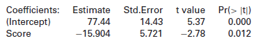
Use the computer output (from different computer packages) to estimate the intercept β0, the slope β1, and to give the equation for the least squares line for the sample. Assume the response variable is Y in each case. Coefficients: Estimate Std.Error t value Pr(> |t) 1.167
Use the computer output (from different computer packages) to estimate the intercept β0, the slope β1, and to give the equation for the least squares line for the sample. Assume the response variable is Y in each case. Coefficients: Estimate Std.Error tvalue Pr(> It)
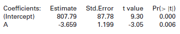
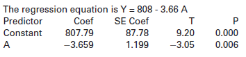
Use the computer output (from different computer packages) to estimate the intercept β0, the slope β1, and to give the equation for the least squares line for the sample. Assume the response variable is Y in each case. The regression equation is Y = 808 - 3.66 A Predictor
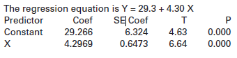
Use the computer output (from different computer packages) to estimate the intercept β0, the slope β1, and to give the equation for the least squares line for the sample. Assume the response variable is Y in each case. The regression equation is Y = 29.3 + 4.30 X Coef 29.266
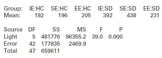
Exercise 6.257 on page 424 introduces a study showing that exercise appears to offer some resiliency against stress, and Exercise 8.18 on page 507 follows up on this introduction. In the study, mice were randomly assigned to live in an enriched environment (EE), a standard environment (SE), or an
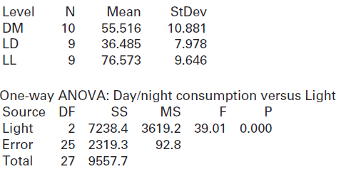
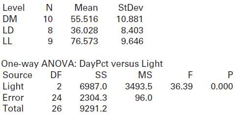
Researchers hypothesized that the increased weight gain seen in mice with light at night might be caused by when the mice are eating. Computer output for the percentage of food consumed during the day (when mice would normally be sleeping) for each of the three light conditions is shown, along with
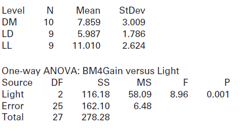
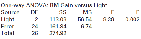
Computer output showing body mass gain (in grams) for the mice after four weeks in each of the three light conditions is shown, along with the relevant ANOVA output. Which light conditions give significantly different mean body mass gain?Data A.1 on page 136 introduces a study in mice showing that
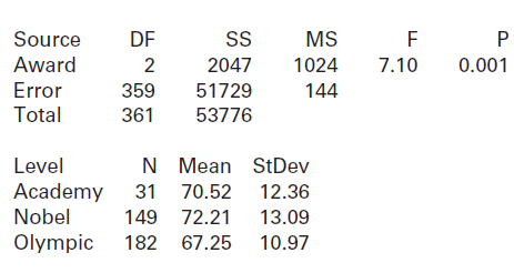
In Example 8.5 on page 500 we find evidence from the ANOVA of a difference in mean pulse rate among students depending on their award preference. The ANOVA table and summary statistics for pulse rates in each group are shown below.Use this information and/or the data in StudentSurvey to compare
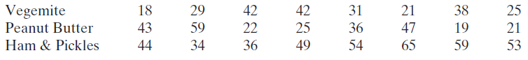
The ANOVA table in Example 8.3 on page 496 for the SandwichAnts data indicates that there is a difference in mean number of ants among the three types of sandwich fillings. In Examples 8.8 and 8.9 we find that the difference is significant between vegemite and ham & pickles, but not between
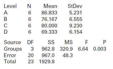
Test for a difference in population means between groups B and D. Show all details of the test.Refer to the data with analysis shown in the following computer output: Level N Mean StDev A 86.833 5.231 76.167 6.555 80.000 9.230 D 69.333 6.154 Source DF Groups SS MS 3 962.8 320.9 6.64 0.003 Error 20
Test for a difference in population means between groups A and B. Show all details of the test.Refer to the data with analysis shown in the following computer output: Level N Mean StDev A 86.833 5.231 76.167 6.555 80.000 9.230 D 69.333 6.154 Source DF Groups SS MS 3 962.8 320.9 6.64 0.003 Error 20
Test for a difference in population means between groups A and D. Show all details of the test.Refer to the data with analysis shown in the following computer output: Level N Mean StDev A 86.833 5.231 76.167 6.555 80.000 9.230 D 69.333 6.154 Source DF Groups SS MS 3 962.8 320.9 6.64 0.003 Error 20
Find a 95% confidence interval for the difference in the means of populations C and D.Refer to the data with analysis shown in the following computer output: Level N Mean StDev A 86.833 5.231 76.167 6.555 80.000 9.230 D 69.333 6.154 Source DF Groups SS MS 3 962.8 320.9 6.64 0.003 Error 20 967.0
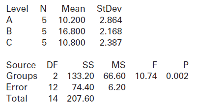
Is there sufficient evidence of a difference in the population means of the three groups? Justify your answer using specific value(s) from the output.Refer to the data with analysis shown in the following computer output: Level N Mean StDev 10.200 2.864 2.168 5 16.800 5 10.800 2.387 Source DF SS MS
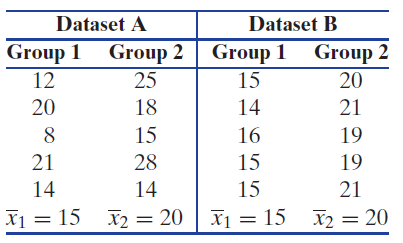
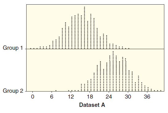
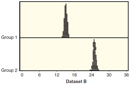
Two sets of sample data, A and B, are given. Without doing any calculations, indicate in which set of sample data, A or B, there is likely to be stronger evidence of a difference in the two population means. Give a brief reason, comparing means and variability, for your answer. Dataset B Dataset A
Find a 99% confidence interval for the mean of population A. Is 90 a plausible value for the population mean of group A?Refer to the data with analysis shown in the following computer output: Level N Mean StDev A 86.833 5.231 76.167 6.555 80.000 9.230 D 69.333 6.154 Source DF Groups SS MS 3 962.8
What is the pooled standard deviation? What degrees of freedom are used in doing inferences for these means and differences in means?Refer to the data with analysis shown in the following computer output: Level N Mean StDev A 86.833 5.231 76.167 6.555 80.000 9.230 D 69.333 6.154 Source DF Groups SS
Is there evidence for a difference in the population means of the four groups? Justify your answer using specific value(s) from the output.Refer to the data with analysis shown in the following computer output: Level N Mean StDev A 86.833 5.231 76.167 6.555 80.000 9.230 D 69.333 6.154 Source DF
Test for a difference in population means between groups A and C. Show all details of the test.Refer to the data with analysis shown in the following computer output: Level N Mean StDev 10.200 2.864 2.168 5 16.800 5 10.800 2.387 Source DF SS MS Groups 2 133.20 66.60 10.74 0.002 Error 12 74.40 6.20
Find a 90% confidence interval for the difference in the means of populations B and C.Refer to the data with analysis shown in the following computer output: Level N Mean StDev 10.200 2.864 2.168 5 16.800 5 10.800 2.387 Source DF SS MS Groups 2 133.20 66.60 10.74 0.002 Error 12 74.40 6.20 Total 14
Find a 95% confidence interval for the mean of population A.Refer to the data with analysis shown in the following computer output: Level N Mean StDev 10.200 2.864 2.168 5 16.800 5 10.800 2.387 Source DF SS MS Groups 2 133.20 66.60 10.74 0.002 Error 12 74.40 6.20 Total 14 207.60
What is the pooled standard deviation? What degrees of freedom are used in doing inferences for these means and differences in means?Refer to the data with analysis shown in the following computer output: Level N Mean StDev 10.200 2.864 2.168 5 16.800 5 10.800 2.387 Source DF SS MS Groups 2 133.20
Most fish use gills for respiration in water and researchers can observe how fast a fish’s gill cover beats to study ventilation, much like we might observe breathing rate for a person. Professor Brad Baldwin is interested in how water chemistry might affect gill beat rates. In one experiment he
In Example 8.5 on page 500 we see a comparison of mean pulse rates between students who prefer each of three different awards (Academy Award, Nobel Prize, Olympic gold medal). The ANOVA test shows that there appears to be a difference in mean pulse rates among those three groups. Can you guess why
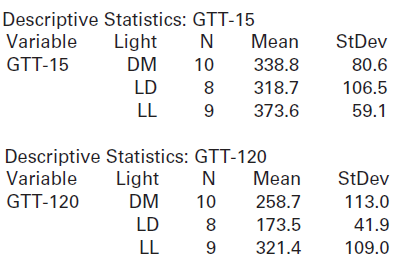
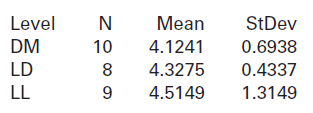
We have seen that light at night increases weight gain in mice and increases the percent of calories consumed when mice are normally sleeping. What effect does light at night have on glucose tolerance? After four weeks in the experimental light conditions, mice were given a glucose tolerance test
Researchers hypothesized that the increased weight gain seen in mice with light at night might be caused by when the mice are eating. (As we have seen in the previous exercises, it is not caused by changes in amount of food consumed or activity level.) Perhaps mice with light at night eat a greater
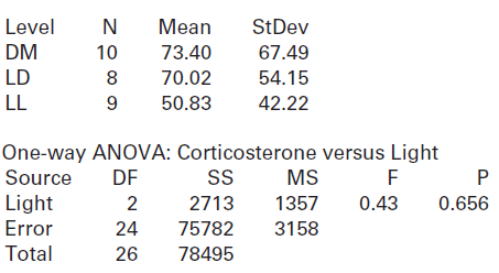
In addition to monitoring weight gain, food consumed, and activity level, the study measured stress levels in the mice by measuring corticosterone levels in the blood (higher levels indicate more stress). Conditions for ANOVA are met and computer output for corticosterone levels for each of the
Perhaps the mice with light at night in Exercise 8.24 are gaining more weight because they are eating more. Computer output is shown for average food consumption (in grams) during week 4 of the study for each of the three light conditions.(a) Is it appropriate to conduct an ANOVA test with these
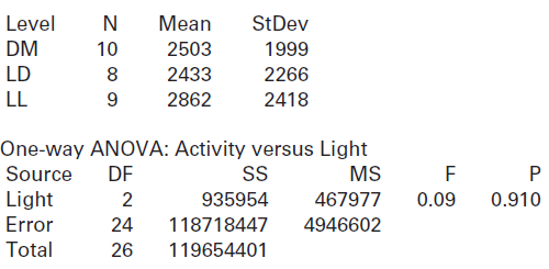
Perhaps the mice with light at night in Exercise 8.24 gain more weight because they are exercising less. The conditions for an ANOVA test are met and computer output is shown for testing the average activity level for each of the three light conditions. Is there a significant difference in mean
The mice in the study had body mass measured throughout the study. Computer output showing an analysis of variance table to test for a difference in mean body mass gain (in grams) after four weeks between mice in the three different light conditions is shown. We see in Exercise 8.24 that the
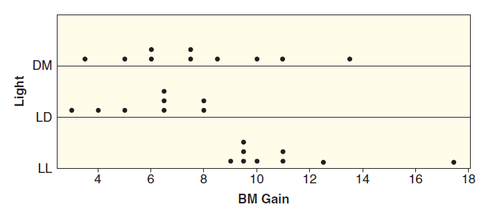
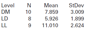
The mice in the study had body mass measured throughout the study. Computer output showing body mass gain (in grams) after 4 weeks for each of the three light conditions is shown, and a dotplot of the data is given inFigure 8.6.(a) In the sample, which group of mice gained the most, on average,
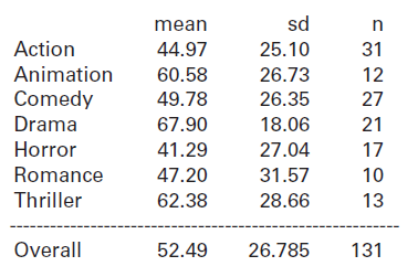
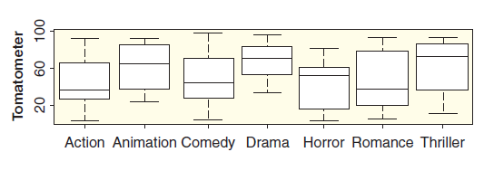
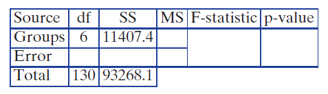
Rotten Tomatoes is a website providing movie ratings and reviews. We have data on all 2011 Hollywood movies, although for this problem we€™ve removed movies classified as €˜€˜Adventure€ or €˜€˜Fantasy€ because there are only
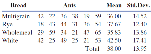
Data 8.1 on page 492 describes an experiment to study how different sandwich fillings might affect the mean number of ants attracted to pieces of a sandwich. The students running this experiment also varied the type of bread for the sandwiches, randomizing between four types: Multigrain, Rye,
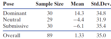
Research shows that people adopting a dominant pose have reduced levels of stress and feel more powerful than those adopting a submissive pose. Furthermore, it is known that if people feel more control over a situation, they have a higher tolerance for pain. Putting these ideas together, a recent
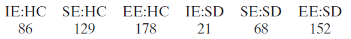
In addition to the behavioral effects of stress, the researchers studied several immunological effects of stress. One measure studied is stress-induced decline in FosB positive cells in the FosB/ΔFosA expression. This portion of the study only included seven mice in each of the six
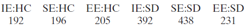
One measure of mouse anxiety is amount of time spent immobile; mice tend to freeze when they are scared. The amount of time (in seconds) spent immobile during one trial is recorded for all the mice and the mean results are shown in Table 8.5.Table 8.5(a) In this sample, do the control groups (HC)
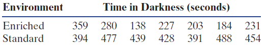
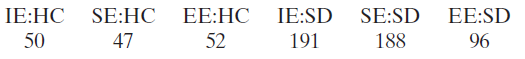
One measure of mouse anxiety is amount of time hiding in a dark compartment, with mice that are more anxious spending more time in darkness. The amount of time (in seconds) spent in darkness during one trial is recorded for all the mice and the results are shown in Table 8.4.Table 8.4(a) In this
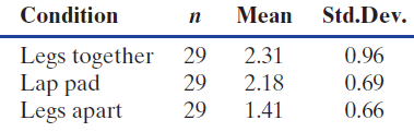
Studies have shown that heating the scrotum by just 1C can reduce sperm count and sperm quality, with long-term consequences. Exercise 2.101 on page 87 introduces a study indicating that males sitting with a laptop on their laps have increased scrotal temperatures. Does a lap pad help reduce the
Color affects us in many ways. For example, Exercise C.51 on page 452 describes an experiment showing that the color red appears to enhance men’s attraction to women. Previous studies have also shown that athletes competing against an opponent wearing red perform worse, and students exposed to
A recent study examined the impact of a mother’s voice on stress levels in young girls. The study included 68 girls ages 7 to 12 who reported good relationships with their mothers. Each girl gave a speech and then solved mental arithmetic problems in front of strangers. Cortisol levels in saliva
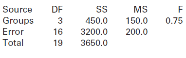
Some computer output for an analysis of variance test to compare means is given.(a) How many groups are there?(b) State the null and alternative hypotheses.(c) What is the p-value?(d) Give the conclusion of the test, using a 5% significance level. Source DF MS Groups 450.0 0.75 3 16 150.0 Error
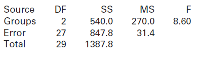
Some computer output for an analysis of variance test to compare means is given.(a) How many groups are there?(b) State the null and alternative hypotheses.(c) What is the p-value?(d) Give the conclusion of the test, using a 5% significance level. Source Groups Error DF MS 540.0 847.8 1387.8 270.0
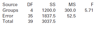
Some computer output for an analysis of variance test to compare means is given.(a) How many groups are there?(b) State the null and alternative hypotheses.(c) What is the p-value?(d) Give the conclusion of the test, using a 5% significance level. Source Groups Error Total SS DF MS 5.71 1200.0
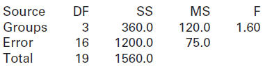
Some computer output for an analysis of variance test to compare means is given.(a) How many groups are there?(b) State the null and alternative hypotheses.(c) What is the p-value?(d) Give the conclusion of the test, using a 5% significance level. Source Groups Error DF SS MS 1.60 120.0 3 360.0 16
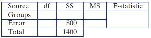
We give sample sizes for the groups in a dataset and an outline of an analysis of variance table with some information on the sums of squares. Fill in the missing parts of the table. What is the value of the F-test statistic?Four groups with n1 = 5, n2 = 8, n3 = 7, and n4 = 5. ANOVA table includes:
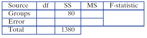
We give sample sizes for the groups in a dataset and an outline of an analysis of variance table with some information on the sums of squares. Fill in the missing parts of the table. What is the value of the F-test statistic?Three groups with n1 = 10, n2 = 8, and n3 = 11. ANOVA table includes:
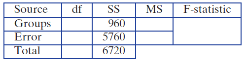
We give sample sizes for the groups in a dataset and an outline of an analysis of variance table with some information on the sums of squares. Fill in the missing parts of the table. What is the value of the F-test statistic?Four groups with n1 = 10, n2 = 10, n3 = 10, and n4 = 10. ANOVA table
Showing 500 - 600
of 2108
1
2
3
4
5
6
7
8
9
10
11
12
13
14
15
Last
Step by Step Answers