New Semester
Started
Get
50% OFF
Study Help!
--h --m --s
Claim Now
Question Answers
Textbooks
Find textbooks, questions and answers
Oops, something went wrong!
Change your search query and then try again
S
Books
FREE
Study Help
Expert Questions
Accounting
General Management
Mathematics
Finance
Organizational Behaviour
Law
Physics
Operating System
Management Leadership
Sociology
Programming
Marketing
Database
Computer Network
Economics
Textbooks Solutions
Accounting
Managerial Accounting
Management Leadership
Cost Accounting
Statistics
Business Law
Corporate Finance
Finance
Economics
Auditing
Tutors
Online Tutors
Find a Tutor
Hire a Tutor
Become a Tutor
AI Tutor
AI Study Planner
NEW
Sell Books
Search
Search
Sign In
Register
study help
business
elementary statistics
Elementary Statistics 3rd Edition William Navidi, Barry Monk - Solutions
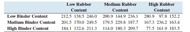
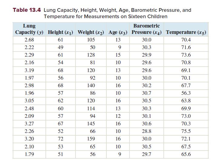
Construct and interpret an interaction plot for the data in Exercise 24.Exercise 24 The following table presents measurements of the tensile strength (in kilopascals) of asphalt-rubber concrete beams for three levels of binder content and three levels of rubber content. Low Binder Content Medium
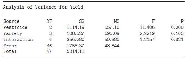
An agricultural scientist performed a two-way ANOVA to determine the effects of three different pesticides on the yield of lemons, in pounds, from four different varieties of lemon tree. The following MINITAB output presents the results.a. Can you reject the hypothesis of no interactions?
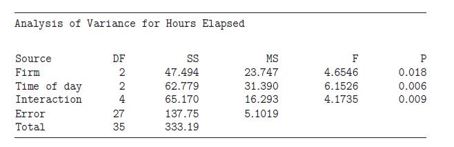
An online retailer sends many packages to customers. To investigate the quality of shipping, the retailer employed three firms to ship packages. Each firm was given four packages to ship at each of three times of day, morning, afternoon, and evening. The outcome variable was the number of hours
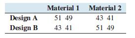
A component can be manufactured according to either of two designs, and with either of two types of material.Two components are manufactured with each combination of design and material, and the lifetimes of each are measured (in hours). The results are as follows.a. Explain why, if one wishes to
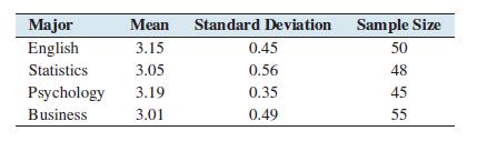
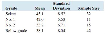
How many degrees of freedom are there for SSTr and for SSE?Exercises 1–4 refer to the following data:At a certain college, random samples of students with various majors were taken, and their grade point averages (GPA) were computed. The following table presents the sample means, standard
Compute the sums of squares SSTr and SSE and the mean squares MSTr and MSE.Exercises 1–4 refer to the following data:At a certain college, random samples of students with various majors were taken, and their grade point averages (GPA) were computed. The following table presents the sample means,
Compute the value of the test statistic F.Exercises 1–4 refer to the following data:At a certain college, random samples of students with various majors were taken, and their grade point averages (GPA)were computed. The following table presents the sample means, standard deviations, and sample
Can you conclude that there are differences in mean GPA among the majors? Use the α = 0.05 level of significance.Exercises 1–4 refer to the following data:At a certain college, random samples of students with various majors were taken, and their grade point averages (GPA)were computed. The
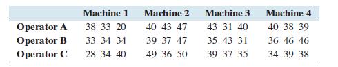
Can you reject the null hypothesis of no interactions? Explain.Exercises 5–7 refer to the following data:A machine shop has four machines used in precision grinding of bearings. Three machinists are employed to grind bearings on the machines. In an experiment to determine whether there are
Can the main effect of operator on the number of parts produced be interpreted? If so, interpret the main effect, using theα = 0.05 level of significance. If not, explain why not.Exercises 5–7 refer to the following data:A machine shop has four machines used in precision grinding of bearings.
Can the main effect of machine on the number of parts produced be interpreted? If so, interpret the main effect, using theα = 0.05 level of significance. If not, explain why not.Exercises 5–7 refer to the following data:A machine shop has four machines used in precision grinding of bearings.
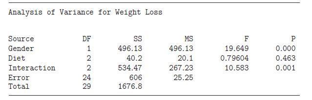
Can you reject the null hypothesis of no interactions? Explain.Exercises 8–10 refer to the following data:As part of a study on weight loss, random samples of men and women were assigned to follow one of three diets. After several weeks, the amount of weight lost, in pounds, was recorded for each
Can the main effect of gender on weight loss be interpreted? If so, interpret the main effect, using the α = 0.01 level of significance. If not, explain why not.Exercises 8–10 refer to the following data:As part of a study on weight loss, random samples of men and women were assigned to follow
Can the main effect of diet on weight loss be interpreted? If so, interpret the main effect, using the α = 0.01 level of significance. If not, explain why not.Exercises 8–10 refer to the following data:As part of a study on weight loss, random samples of men and women were assigned to follow one
A certain experiment consisted of I = 5 treatments, with sample sizes n1 = n2 = n3 = n4 = n5 = 4.The sums of squares were SSTr = 43.7 and SSE = 79.8.a. How many degrees of freedom are there for SSTr?b. How many degrees of freedom are there for SSE?c. Find the treatment mean square MSTr.d. Find the
A certain experiment consisted of I = 3 treatments, with sample sizes n1 = n2 = n3 = 5.The sums of squares were SSTr = 7.3 and SSE = 3.9.a. How many degrees of freedom are there for SSTr?b. How many degrees of freedom are there for SSE?c. Find the treatment mean square MSTr.d. Find the error mean
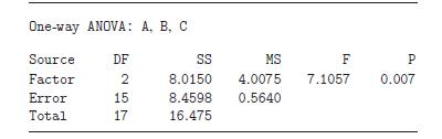
The following MINITAB output presents the results of a one-way ANOVA.a. State the null hypothesis.b. How many levels were there for the factor?c. Assume the design was balanced. What was the sample size for each factor?d. What are the values of SSTr, SSE, MSTr, and MSE?e. What is the value of the
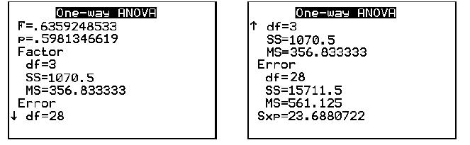
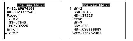
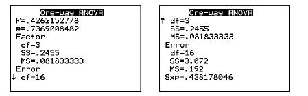
The following TI-84 Plus display presents the results of a one-way ANOVA.a. State the null hypothesis.b. How many levels were there for the factor?c. Assume the design was balanced. What was the sample size for each factor?d. What are the values of SSTr, SSE, MSTr, and MSE?e. What is the value of
In a one-way ANOVA with three samples, the sample means were ̄x1 = 24.03,̄x2 = 14.88, and ̄x3 = 12.76. The sample sizes were n1 = n2 = n3 = 6, and the error mean square was MSE = 10.53. Perform the Tukey–Kramer test on each pair of means. Which pairs can you conclude to be different? Use the
In a one-way ANOVA with four samples, the sample means were ̄x1 = 86.8,̄x2 = 82.4, ̄x3 = 85.8, and ̄x4 = 89.1. The sample sizes were n1 = n2 = n3 = n4 = 4, and the error mean square was MSE = 1.3. Perform the Tukey–Kramer test on each pair of means. Which pairs can you conclude to be
In one-way ANOVA, the null hypothesis states that all the population means are __________________ .In Exercises 7 and 8, fill in each blank with the appropriate word or phrase.
In one-way ANOVA, the effect of unequal variances can be substantial when the design is ____________________ .In Exercises 7 and 8, fill in each blank with the appropriate word or phrase.
If the sample means are widely spread, the value of SSTr will tend to be large.In Exercises 9–12, determine whether the statement is true or false. If the statement is false, rewrite it as a true statement.
In one-way ANOVA, all the samples must be the same size.In Exercises 9–12, determine whether the statement is true or false. If the statement is false, rewrite it as a true statement.
In one-way ANOVA, we have samples from several populations.In Exercises 9–12, determine whether the statement is true or false. If the statement is false, rewrite it as a true statement.
If the sample means are widely spread, the value of SSE will tend to be large.In Exercises 9–12, determine whether the statement is true or false. If the statement is false, rewrite it as a true statement.
In a one-way ANOVA, the following data were collected:SSTr = 0.25, SSE = 2.11, N = 34, I = 4.a. How many samples are there?b. How many degrees of freedom are there for SSTr and SSE?c. Compute the mean squares MSTr and MSE.d. Compute the value of the test statistic F.e. Can you conclude that two or
In a one-way ANOVA, the following data were collected:SSTr = 145.34, SSE = 38.45, N = 9, I = 3.a. How many samples are there?b. How many degrees of freedom are there for SSTr and SSE?c. Compute the mean squares MSTr and MSE.d. Compute the value of the test statistic F.e. Can you conclude that two
Samples were drawn from three populations. The sample sizes were n1 = 8, n2 = 6, n3 = 9.The sample means were ̄x1 = 1.04,̄x2 = 1.25, ̄x3 = 1.87. The sample standard deviations were s1 = 0.25, s2 = 0.43, s3 = 0.34. The grand mean was x̄̄ = 1.42.a. Compute the sums of squares SSTr and SSE.b. How
Samples were drawn from four populations. The sample sizes were n1 = 9, n2 = 7, n3 = 10, n4 = 8.The sample means werēx1 = 73.5, ̄x2 = 74.8, ̄x3 = 75.1, ̄x4 = 78.2. The sample standard deviations were s1 = 2.5, s2 = 4.5, s3 = 3.8, s4 = 3.2. The grand mean was x̄̄ = 75.34.a. Compute the sums
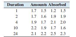
One of the factors that determines the degree of risk a pesticide poses to human health is the rate at which the pesticide is absorbed into skin after contact. An important question is whether the amount in the skin continues to increase with the length of the contact, or whether it increases for
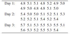
Penicillin is produced by the Penicillium fungus, which is grown in a broth whose sugar content must be carefully controlled. Several samples of broth were taken on three successive days, and the amount of dissolved sugars, in milligrams per milliliter, was measured on each sample. The results were
Using the data in Exercise 17, perform the Tukey–Kramer test to determine which pairs of means, if any, differ. Use the α = 0.05 level of significance.Exercise 17One of the factors that determines the degree of risk a pesticide poses to human health is the rate at which the pesticide is absorbed
Using the data in Exercise 18, perform the Tukey–Kramer test to determine which pairs of means, if any, differ. Use the α = 0.05 level of significance.Exercise 18Penicillin is produced by the Penicillium fungus, which is grown in a broth whose sugar content must be carefully controlled. Several
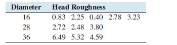
Artificial hip joints consist of a ball and socket.As the joint wears, the ball (head) becomes rough. Investigators performed wear tests on metal artificial hip joints. Joints with several different diameters were tested. The following table presents measurements of head roughness (in
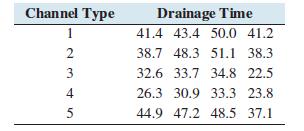
Rapid drainage of floodwater is crucial to prevent damage during heavy rains. Several designs for a drainage canal were considered for a certain city. Each design was tested five times, to determine how long it took to drain the water in a reservoir. The following table presents the drainage times,
Using the data in Exercise 21, perform the Tukey–Kramer test to determine which pairs of means, if any, differ. Use the α = 0.01 level of significance.Exercise 21Artificial hip joints consist of a ball and socket.As the joint wears, the ball (head) becomes rough. Investigators performed wear
Using the data in Exercise 22, perform the Tukey–Kramer test to determine which pairs of means, if any, differ. Use the α = 0.01 level of significance.Exercise 22Rapid drainage of floodwater is crucial to prevent damage during heavy rains. Several designs for a drainage canal were considered for
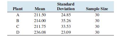
Power plants can emit levels of pollution that can lower air quality. For this reason, it is important to monitor the levels of pollution they produce.Investigators measured dust emissions, in milligrams per cubic meter, at four power plants. Thirty measurements were taken for each plant. The
The strength of wood products used in construction is measured to be sure that they are suitable for the purpose for which they are used. Measurements, in megapascals, of the strength needed to break green mixed oak boards were made. The sample means, standard deviations, and sample sizes for four
Several large-sized sodas were ordered at each of several fast-food restaurants, and the volume of beverage in each was measured. The following TI-84 Plus display presents the results of a one-way ANOVA to determine whether the mean volume differs among the restaurants.a. State the null
Several spreadsheet programs were tested by performing a certain task several times on each. The following TI-84 Plus display presents the results of a one-way ANOVA to determine whether the mean time required to perform a certain task differs among them.a. State the null hypothesis.b. How many
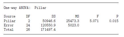
Automotive engineers compared three types of A-pillars in automobiles to determine which provided the greatest protection to occupants of automobiles during a collision. Following is a one-way ANOVA table. The response variable is the head injury criterion (HIC), which is a number that measures the
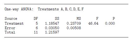
High levels of phosphorus in soil can lead to severe reductions in water quality and animal populations.Investigators treated soil specimens with six different treatments, and the acid phosphatase activity, which is related to the production of phosphorus, was recorded. Results are presented in the
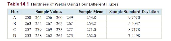
Refer to Table 14.1, which presents data on the hardnesses of welds produced from four different fluxes.a. There are six possible hypotheses to test regarding pairs of fluxes. They are: H0: μ1 − μ2 = 0, H0: μ1 − μ3 = 0, H0: μ1 − μ4 = 0, H0: μ2 − μ3 = 0, H0: μ2 − μ4 = 0, and H0:
The following MINITAB output presents a multiple regression equation̂y = b0 + b1x1 + b2x2 + b3x3 + b4x4.It is desired to drop one of the explanatory variables. Which of the following is the most appropriate action?i. Drop x1, then see whether R2 increases.ii. Drop x2, then see whether adjusted R2
For a sample of size n = 20, the following values were obtained: b0 = 1.05, b1 = 4.50, se = 0.54, ∑(x − x̄ )2 = 10.9, x̄ = 8.52. Construct a 95% confidence interval for the mean response when x = 10.
For a sample of size n = 15, the following values were obtained: b0 = 3.71, b1 = 8.38, se = 1.13, ∑(x − x̄)2 = 7.71, x̄ = 13.16. Construct a 95% prediction interval for an individual response when x = 8.
A _______________ interval estimates the mean y-value for all individuals with a given x-value.In Exercises 3 and 4, fill in each blank with the appropriate word or phrase.
A _______________ interval estimates the y-value for a particular individual with a given x-value.In Exercises 3 and 4, fill in each blank with the appropriate word or phrase.
For a given x-value, the 95% confidence interval for the mean response will always be wider than the 95% prediction interval.In Exercises 5 and 6, determine whether the statement is true or false. If the statement is false, rewrite it as a true statement.
For a given x-value, the point estimate for a 95% confidence interval for the mean response is the same as the one for the 95% prediction interval.In Exercises 5 and 6, determine whether the statement is true or false. If the statement is false, rewrite it as a true statement.
For a sample of size 25, the following values were obtained:b0 = 3.25, b1 = 2.32, se = 3.53, ∑(x − ̄x)2 = 224.05, and̄x = 0.98.a. Construct a 95% confidence interval for the mean response when x = 2.b. Construct a 95% prediction interval for an individual response when x = 2.
For a sample of size 18, the following values were obtained:b0 = 2.27, b1 = −1.46, se = 5.72, ∑(x − ̄x)2 = 360.26, and̄x = 1.95.a. Construct a 99% confidence interval for the mean response when x = 2.b. Construct a 99% prediction interval for an individual response when x = 2.
In Exercises 9 and 10, use the given set of points toa. Compute b0 and b1.b. Compute the predicted value ̂y for the given value of x.c. Compute the residual standard deviation se.d. Compute the sum of squares for x, ∑(x − ̄x)2.e. Find the critical value for a 95% confidence or prediction
In Exercises 9 and 10, use the given set of points toa. Compute b0 and b1.b. Compute the predicted value ̂y for the given value of x.c. Compute the residual standard deviation se.d. Compute the sum of squares for x, ∑(x − ̄x)2.e. Find the critical value for a 95% confidence or prediction
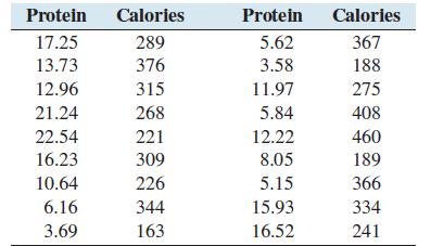
Use the data in Exercise 19 in Section 13.1 for the following:a. Compute a point estimate for the mean number of calories in fast-food products that contain 15 grams of protein.b. Construct a 95% confidence interval for the mean number of calories in fast-food products that contain 15 grams of
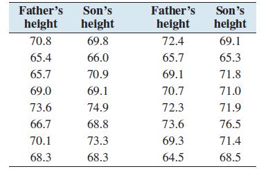
Use the data in Exercise 20 in Section 13.1 for the following.a. Compute a point estimate of the mean height of sons whose fathers are 70 inches tall.b. Construct a 95% confidence interval for the mean height of sons whose fathers are 70 inches tall.c. Predict the height of a particular son whose
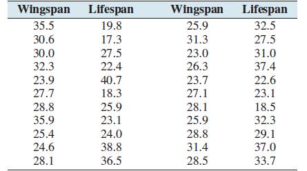
Use the data in Exercise 21 in Section 13.1 for the following.a. Compute a point estimate of the mean lifespan of butterflies with a wingspan of 30 millimeters.b. Construct a 95% confidence interval for the mean lifespan of butterflies with a wingspan of 30 millimeters.c. Predict the lifespan of a
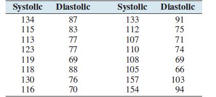
Use the data in Exercise 22 in Section 13.1 for the following.a. Compute a point estimate of the mean diastolic pressure for people whose systolic pressure is 120.b. Construct a 95% confidence interval for the mean diastolic pressure for people whose systolic pressure is 120.c. Predict the
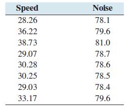
Use the data in Exercise 23 in Section 13.1 for the following.a. Compute a point estimate for the mean noise level for streets with a mean speed of 35 kilometers per hour.b. Construct a 99% confidence interval for the mean noise level for streets with a mean speed of 35 kilometers per hour.c.
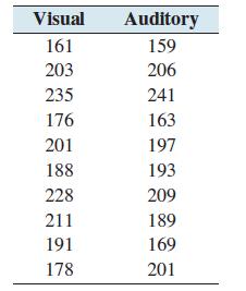
Use the data in Exercise 24 in Section 13.1 for the following.a. Compute a point estimate for the mean auditory response time for subjects with a visual response time of 200.b. Construct a 99% confidence interval for the mean auditory response time for subjects with a visual response time of 200.c.
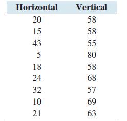
Use the data in Exercise 25 in Section 13.1 for the following.a. Compute a point estimate for the mean vertical expansion at locations where the horizontal expansion is 25.b. Construct a 99% confidence interval for the mean vertical expansion at locations where the horizontal expansion is 25.c.
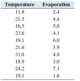
Use the data in Exercise 26 in Section 13.1 for the following.a. Compute a point estimate for the mean evaporation rate when the temperature is 20°C.b. Construct a 99% confidence interval for the mean evaporation rate for all days with a temperature of 20°C.c. Predict the evaporation rate when
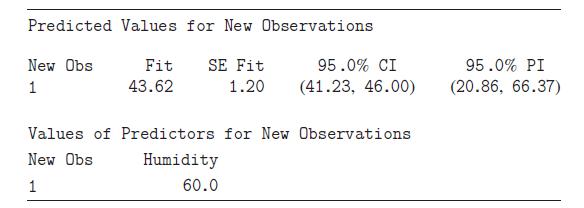
The following MINITAB output presents a 95%confidence interval for the mean ozone level on days when the relative humidity is 60%, and a 95% prediction interval for the ozone level on a particular day when the relative humidity is 60%. The units of ozone are parts per billion.a. What is the point
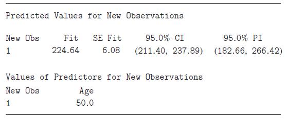
The following MINITAB output presents a 95%confidence interval for the mean cholesterol levels for men aged 50 years, and a 95% prediction interval for an individual man aged 50.The units of cholesterol are milligrams per deciliter.a. What is the point estimate for the mean cholesterol level for
Several 95% confidence intervals for the mean response will be constructed, based on a data set for which the sample mean value for the explanatory variable is̄x = 10.The values of x∗ for which the confidence intervals will be constructed are x* = 9, x* = 12, and x* = 14.a. For which of these
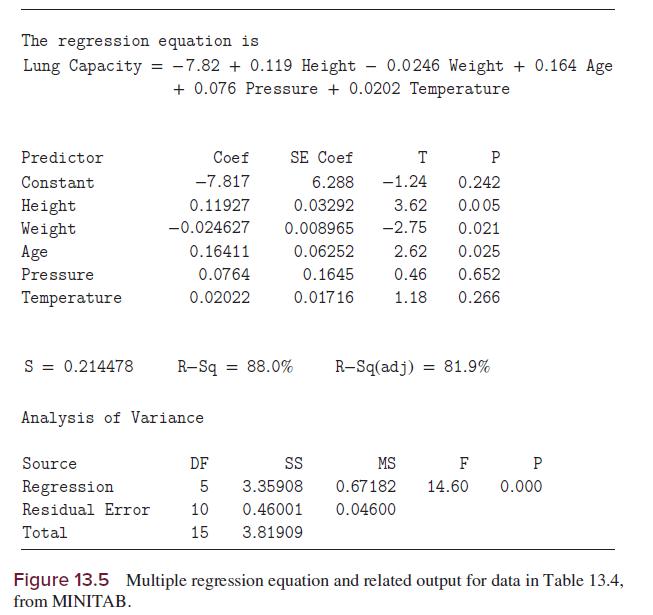
Use the coefficients of the multiple regression equation in Figure 13.5 to predict the lung capacity for a 10-year-old who is 57 inches tall and weighs 90 pounds, at a pressure of 30.2 inches and a temperature of 65 degrees. The regression equation is Lung Capacity = -7.82 0.119 Height - 0.0246
Two people differ in age by 1.5 years. Their heights and weights are the same, and their lung capacities are measured at the same pressure and temperature. By how much should we predict their lung capacities to differ?
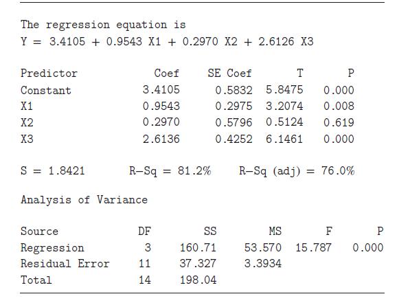
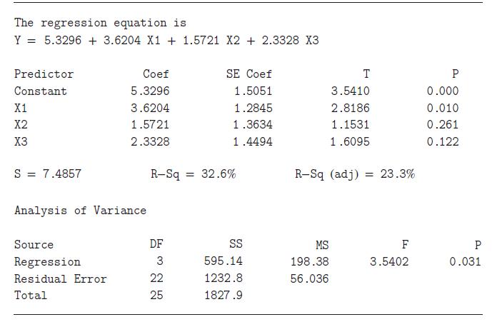
The following MINITAB output presents a multiple regression equation̂y = b0 + b1x1 + b2x2 + b3x3. Test H0 : βi = 0 versus H1: βi ≠ 0 for i = 1, 2, 3.Use theα = 0.05 level. The regression equation is Y3.4105 +0.9543 X1 +0.2970 X2 + 2.6126 X3 Predictor Coef SE Coef T _ P Constant 3.4105 0.5832
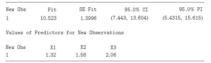
The following MINITAB output presents a confidence interval for a mean response and a prediction interval for an individual response.a. Predict the value of y when x1 = 1.32, x2 = 1.58, and x3 = 2.06.b. We are 95% confident that an individual whose values are x1 = 1.32, x2 = 1.58, and x3 = 2.06
The following MINITAB output presents a multiple regression equation.a. What percentage of the variation in the response is explained by the multiple regression equation?b. What percentage of the variation in the response is explained by the multiple regression equation, if we account for the
Refer to Exercise 5.a. Is the multiple regression equation useful for prediction? Explain. Use theα = 0.05 level.b. Is the multiple regression equation useful for prediction? Explain. Use theα = 0.01 level.Exercise 5The following MINITAB output presents a multiple regression equation. The
A _____________ plot can be used to determine whether a multiple regression equation is appropriate.In Exercises 7 and 8, fill in each blank with the appropriate word or phrase.
We should leave a variable out of a multiple regression equation when removing it ______________ the value of adjusted R2.In Exercises 7 and 8, fill in each blank with the appropriate word or phrase.
The coefficient of determination R2 measures the percentage of variation in the outcome that is explained by the model.In Exercises 9 and 10, determine whether the statement is true or false. If the statement is false, rewrite it as a true statement.
If the value of the F-statistic is large, the multiple regression equation is not useful for making predictions.In Exercises 9 and 10, determine whether the statement is true or false. If the statement is false, rewrite it as a true statement.
For the following data set: a. Construct the multiple regression equation ̂y = b0 + b1x1 + b2x2 + b3x3.b. Predict the value of y when x1 = 1, x2 = 4.5, x3 = 6.2.c. What percentage of the variation in y is explained by the model?d. Is the model useful for prediction? Why or why not? Use the α =
For the following data set:a. Construct the multiple regression equationb. Predict the value of y when x1 = 10.1, x2 = 8.5, x3 = 26.2.c. What percentage of the variation in y is explained by the model?d. Is the model useful for prediction? Why or why not? Use the α = 0.05 level.e. Test H0: β1 = 0
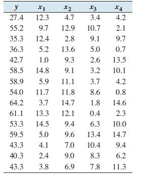
For the following data set:a. Construct the multiple regression equationb. Predict the value of y when x1 = 5.2, x2 = 9.1, x3 = 8.7, x4 = 2.8.c. What percentage of the variation in y is explained by the model?d. Is the model useful for prediction? Why or why not? Use the α = 0.01 level.e. Test H0:
For the following data set:a. Construct the multiple regression equationb. Predict the value of y when x1 = 15.3, x2 = 4.7, x3 = 0.6, x4 = 8.2.c. What percentage of the variation in y is explained by the model?d. Is the model useful for prediction? Why or why not? Use the α = 0.05 level.e. Test
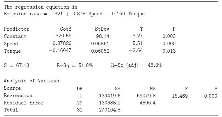
In a laboratory test of a new automobile engine design carried out at the Colorado School of Mines, the emission rate (in milligrams per second) of oxides of nitrogen was measured for 32 engines at various engine speeds (in rpm) and engine torque (in foot-pounds). The following MINITAB output
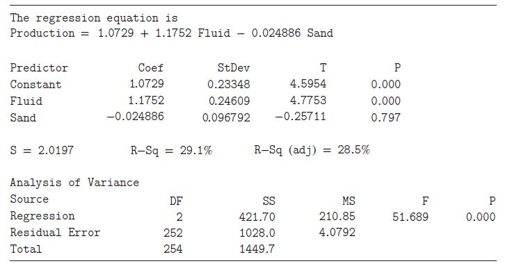
Natural gas is found in rock formations underground. In order to extract the gas, a procedure known as hydraulic fracturing, or‘‘fracking,’’ is often used. In this procedure, fluid mixed with sand is pumped into the gas well and forced through cracks in the rock. The sand holds open the
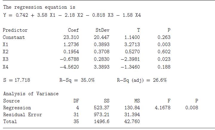
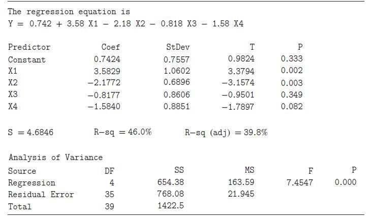
The following MINITAB output presents a multiple regression equation ̂y = b0 + b1x1 + b2x2 + b3x3 + b4x4.It is desired to drop one of the explanatory variables. Which of the following is the most appropriate action?i. Drop x3, then see whether R2 increases.ii. Drop x3, then see whether adjusted R2
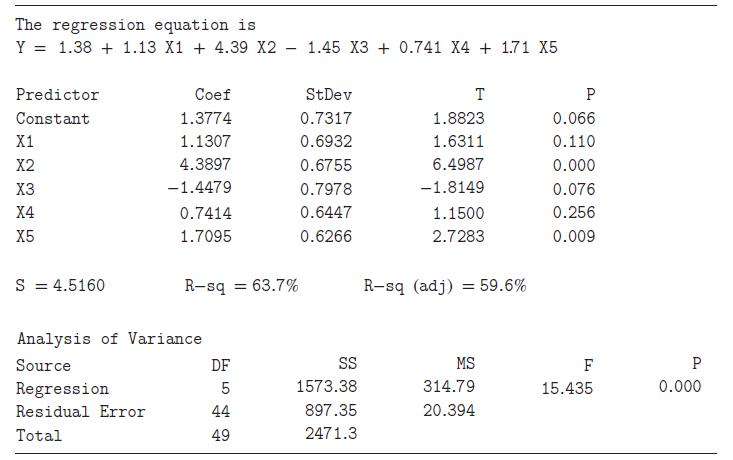
The following MINITAB output presents a multiple regression equation ̂y = b0 + b1x1 + b2x2 + b3x3 + b4x4 + b5x5.It is desired to drop one of the explanatory variables. Which of the following is the most appropriate action?i. Drop x2, then see whether R2 increases.ii. Drop x4, then see whether R2
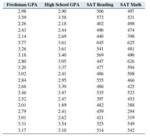
Twenty college students were sampled after their freshman year. Following are their freshman GPAs, their high school GPAs, their SAT reading scores, and their SAT math scores.a. Let y represent freshman GPA, x1 represent high school GPA, x2 represent SAT reading score, and x3 represent SAT math
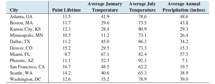
A paint company collected data on the lifetime (in years) of its paint in eleven United States cities. The data are in the following table.a. Let y represent paint lifetime, x1 represent January temperature, x2 represent July temperature, and x3 represent annual precipitation.Construct the multiple
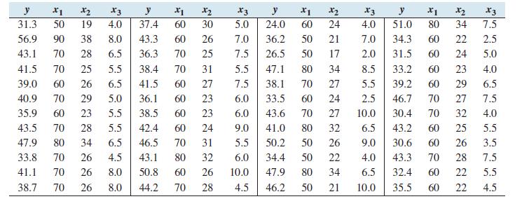
A chemical reaction was run 48 times. In each run, different values were chosen for the temperature in degrees Celsius(x1), the concentration of the primary reactant (x2), and the number of hours the reaction was allowed to run (x3). The outcome variable (y)is the amount of product.a. Construct the
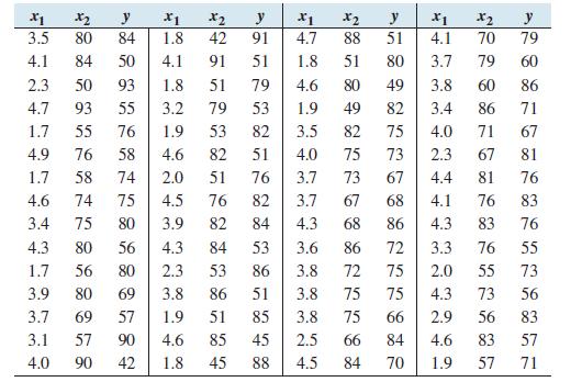
The following table lists values measured for 60 consecutive eruptions of the geyser Old Faithful in Yellowstone National Park. They are the duration of the eruption (x1), the duration of the dormant period immediately before the eruption (x2), and the duration of the dormant period immediately
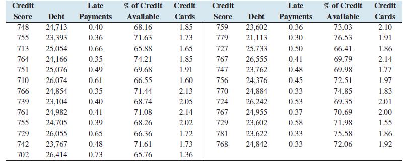
Credit data were collected on a random sample of 25 U.S. cities in a recent year. Following are the average credit scores, the average debt, the average number of late payments, the average percentage of credit available, and the average number of open credit cards.a. Let y represent average credit
A confidence interval for β1 is to be constructed from a sample of 20 points. How many degrees of freedom are there for the critical value?
A confidence interval for a mean response and a prediction interval for an individual response are to be constructed from the same data. True or false: The number of degrees of freedom for the critical value is the same for both intervals.
True or false: If we fail to reject the null hypothesis H0: β1 = 0, we can conclude that there is no linear relationship between the explanatory variable and the outcome variable.
True or false: When the sample size is large, confidence intervals and hypothesis tests for β1 are valid even when the assumptions of the linear model are not met.
A statistics student has constructed a confidence interval for the mean height of daughters whose mothers are 66 inches tall, and a prediction interval for the height of a particular daughter whose mother is 66 inches tall. One of the intervals is (65.3, 68.2) and the other is (63.8, 69.7).
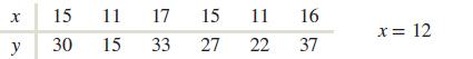
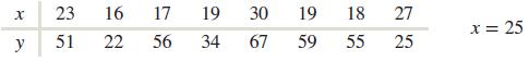
Compute the point estimates b0 and b1.Exercises 6–10 refer to the following data set: x 25 13 16 19 29 19 16 30 y 40 20 33 30 50 37 34 37
Construct a 95% confidence interval for β1.Exercises 6–10 refer to the following data set: x 25 13 16 19 29 19 16 30 y 40 20 33 30 50 37 34 37
Test the hypotheses H0: β1 = 0 versus H1: β1 ≠ 0.Use the α = 0.01 level of significance.Exercises 6–10 refer to the following data set: x 25 13 16 19 29 19 16 30 y 40 20 33 30 50 37 34 37
Construct a 95% confidence interval for the mean response when x = 20.Exercises 6–10 refer to the following data set: x 25 13 16 19 29 19 16 30 y 40 20 33 30 50 37 34 37
Construct a 95% prediction interval for an individual response when x = 20.Exercises 6–10 refer to the following data set: x 25 13 16 19 29 19 16 30 y 40 20 33 30 50 37 34 37
Showing 5400 - 5500
of 7930
First
48
49
50
51
52
53
54
55
56
57
58
59
60
61
62
Last
Step by Step Answers