Questions and Answers of Control Systems Engineering

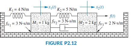
For the system of Figure P2.12 find the transfer function, G(s) = X1(s)/F(s). K = 4 N/m -Xj K, = 5 N/m ft) = 3 N-s/mM1 =T'kg Jv2=3N-s/m M2 = 2 kg fva = 2 N-s/m %3D FIGURE P2.12
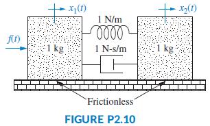
Find the transfer function, G(s) = X2(s)/F(s), for the translational mechanical network shown in Figure P2.10. X(1) X(1) 1 N/m ft) 1 kg 1 N-s/m 1 kg Frictionless" FIGURE P2.10
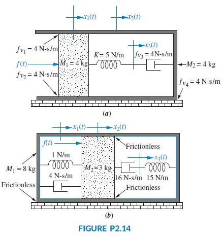
Find the transfer function, X3(s)/F(s), for each system shown in Figure P2.14. 13() fv = 4 N-s/mp K= 5 N/m fv = 4N-s/m f()- M, = 4 kg0000 M2 = 4 kg fvz = 4 N-s/m fv=4 N-s/m (a) X(1) Frictionless 1
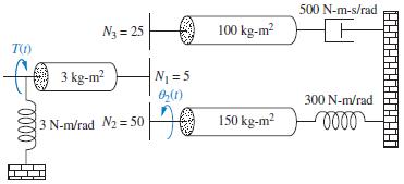
Find the transfer function, G(s) = θ2(s)/T(s), for the rotational mechanical system shown in Figure P2.22. 500 N-m-s/rad N3 = 25 100 kg-m? 3 kg-m? N1 = 5 300 N-m/rad 3 N-m/rad N2 = 50 150 kg-m?
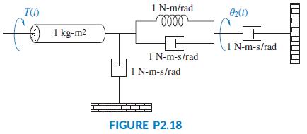
For the rotational mechanical system shown in Figure P2.18, find the transfer function G(s) = θ2(s)/T(s) 1 N-m/rad T(1t) O2(1) 1 kg-m2 1 N-m-s/rad 1 N-m-s/rad 1 N-m-s/rad FIGURE P2.18
Asystem’s output, c, is related to the system’s input, r, by the straight-line relationship, c = 5r + 7. Is the system linear?
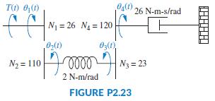
Find the transfer function, G(s) = θ4(s)/T(s), for the rotational system shown in Figure P2.23. O0) 26 N-m-s/rad N1 = 26 N4 = 120 N2 = 110 N3 = 23 2 N-m/rad FIGURE P2.23
Consider the differential equationwhere f(x) is the input and is a function of the output, x. If f (x) = sin x, linearize the differential equation for small excursions. [Section: 2.10]a. x = 0b. x =
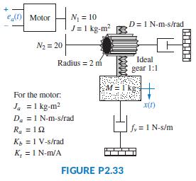
Find the transfer function, G(s) = X(s)/Ea(s), for the system shown in Figure P2.33. + e(n Motor N = 10 J= 1 kg-m? 3 D=1 N-m-s/rad N2 = 20 Radius = 2 m Ideal gear 1:1 M=I'kg For the motor: J. =1
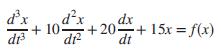
Consider the differential equationwhere f(x) is the input and is a function of the output, x. If f (x) = 3e-5x, linearize the differential equation for x near 0. d'x dr + 10+ dx dx + 20+ 15x = f(x)
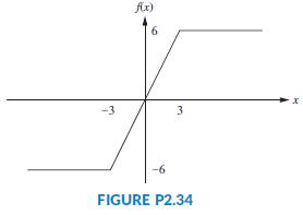
Many systems are piecewise linear. That is, over a large range of variable values, the system can be described linearly. A system with amplifier saturation is one such example. Given the differential
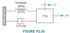
For the translational mechanical system with a nonlinear spring shown in Figure P2.35, find the transfer function, G(s) = X(s)/F(s), for small excursions around f (t) = 1. The spring is defined by
Enzymes are large proteins that biological systems use to increase the rate at which reactions occur. For example, food is usually composed of large molecules that are hard to digest; enzymes break
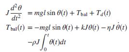
Humans are able to stand on two legs through a complex feedback system that includes several sensory inputs— equilibrium and visual along with muscle actuation. In order to gain a better
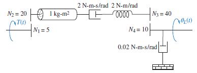
For the rotational system shown in Figure P2.24, find the transfer function, G(s) = θL(s)/T(s).Figure P2.24 2 N-m-s/rad 2 N-m/rad N2 = 20 A 1 kg-m2 E0000 N3 = 40 N1 = 5 N4= 10 0.02 N-m-s/rad
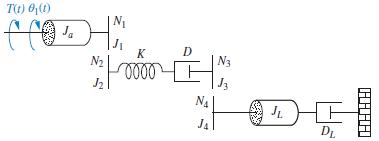
For the rotational system shown in Figure P2.25, write the equations of motion from which the transfer function, G(s) = θ1(s)/T(s), can be found.Figure P2.25 T(t) 0,(1) N J. K D N2 N3 J2 N4
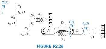
Given the rotational system shown in Figure P2.26, find the transfer function, G(s) = θ6(s)/θ1(s). J1, D N2 K1 Na Jz D N4 J6 Js 000 D K2 FIGURE P2.26
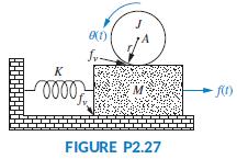
In the system shown in Figure P2.27, the inertia, J, of radius, r, is constrained to move only about the stationary axis A. A viscous damping force of translational value fv exists between the bodies
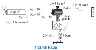
For the combined translational and rotational system shown in Figure P2.28, find the transfer function, G(s) = X(s)/T(s). J= 3 kg-m? B Radius = 2 m 1 N-m-s/rad TO) N = 10 A 3 kg-m2 N2 = 20 N4 = 60
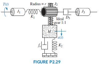
Given the combined translational and rotational system shown in Figure P2.29, find the transfer function, G(s) = X(s)/T(s). T(O) Radius = r Bh 0000 Ideal D3 gear 1:1 K2 FIGURE P2.29
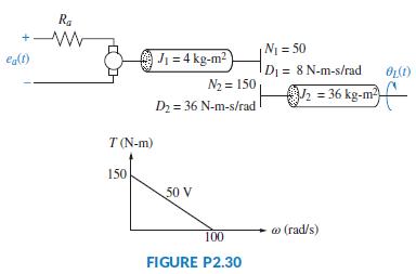
For the motor, load, and torque-speed curve shown in Figure P2.30, find the transfer function, G(s) = θL(s)/Ea(s). Ra N = 50 ea(t) J = 4 kg-m2 D = 8 N-m-s/rad N2 = 150 = 36 kg-m D2 = 36 N-m-s/rad T
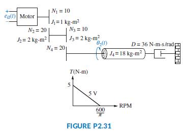
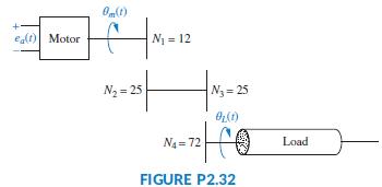
The motor whose torque-speed characteristics are shown in Figure P2.31 drives the load shown in the diagram. Some of the gears have inertia. Find the transfer function, G(s) = θ2(s)=Ea(s). N1 = 10
A dc motor develops 55 N-m of torque at a speed of 600 rad/s when 12 volts are applied. It stalls out at this voltagewith100N-mof torque. If the inertia and damping of the armature are7kg-m2 and
In this chapter, we derived the transfer function of a dc motor relating the angular displacement output to the armature voltage input. Often we want to control the output torque rather than the
How can you tell from the root locus if the settling time does not change over a region of gain?
The characteristic polynomial of a feedback control system, which is the denominator of the closed-loop transfer function, is given by s3 + 2s2 + (20K + 7)s + 100K. Sketch the root locus for this
How can you tell from the root locus that the natural frequency does not change over a region of gain?
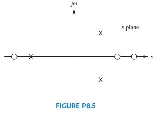
Figure P8.5 shows open-loop poles and zeros. There are two possibilities for the sketch of the root locus. Sketch each of the two possibilities. Be aware that only one can be the real locus for
How would you determine whether or not a root locus plot crossed the real axis?
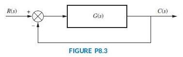
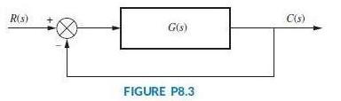
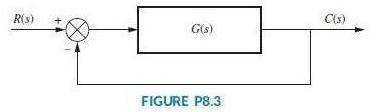
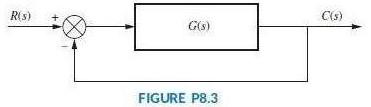
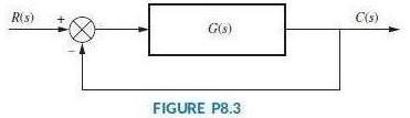
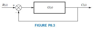
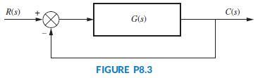
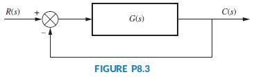
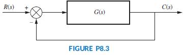
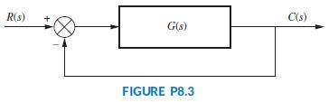
Plot the root locus for the unity feedback system shown in Figure P8.3, whereFor what range of K will the poles be in the right half-plane? K(s + 2)(s + 4) G(s) = (s+5)(s – 3)
Describe the conditions that must exist for all closed-loop poles and zeros in order to make a second-order approximation.
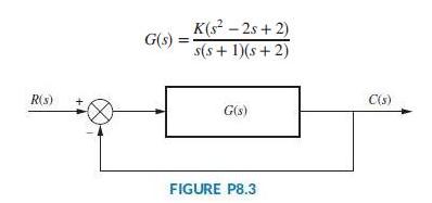
For the unity feedback system shown in Figure P8.3, wheresketch the root locus and tell for what values of K the system is stable and unstable. K(s-9) G(s) = (s2 +4)
What rules for plotting the root locus are the same whether the system is a positive- or a negative-feedback system?
Sketch the root locus for the unity feedback system shown in Figure P8.3, whereGive the values for all critical points of interest. Is the system ever unstable? If so, for what range of K? K(s² +2)
Briefly describe how the zeros of the open-loop system affect the root locus and the transient response.
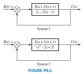
For each system shown in Figure P8.6, make an accurate plot of the root locus and find the following:a. The breakaway and break-in pointsb. The range of K to keep the system stablec. The value of K
Sketch the root locus and find the range of K for stability for the unity feedback system shown in Figure P8.3 for the following conditions:a.b. K(s? + 1) G(s) (s - 1)(s+2)(s+ 3)
For the unity feedback system of Figure P8.3, wheresketch the root locus and find the range of K such that there will be only two right–half-plane poles for the closed-loop system. K(s + 5) (s2 +
For the unity feedback system of Figure P8.3, whereplot the root locus and calibrate your plot for gain. Find all the critical points, such as breakaways, asymptotes, jω-axis crossing, and so forth.
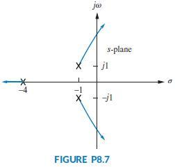
Given the root locus shown in Figure P8.7,a. Find the value of gain that will make the system marginally stable.b. Find the value of gain for which the closed-loop transfer function will have a pole
Given the unity feedback system of Figure P8.3, make an accurate plot of the root locus for the following:a.b.Also, do the following:Calibrate the gain for at least four points for each case. Also
Given the unity feedback system of Figure P8.3, wheredo the following:a. Sketch the root locus.b. Find the asymptotes.c. Find the value of gain that will make the system marginally stable.d. Find the
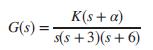
For the unity feedback system of Figure P8.3, wherefind the values of α and K that will yield a second-order closed-loop pair of poles at -1 ± j100. K(s + a) G(s) s(s +3)(s + 6)
For the unity feedback system of Figure P8.3, wheresketch the root locus and find the following:a. The breakaway and break-in pointsb. The jω-axis crossingc. The range of gain to keep the system
For the unity feedback system shown in Figure P8.3, wheredo the following:a. Sketch the root locus.b. Find the range of gain, K, that makes the system stable.c. Find the value of K that yields a
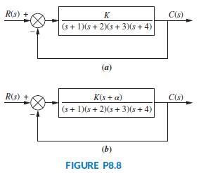
For the system of Figure P8.8(a), sketch the root locus and find the following:a. Asymptotesb. Breakaway pointsc. The range of K for stabilityd. The value of K to yield a 0.7 damping ratio for the
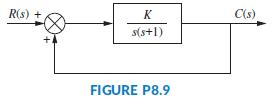
Sketch the root locus for the positive-feedback system shown in Figure P8.9. R(s) + K C(s) s(s+1) FIGURE P8.9
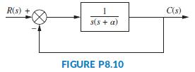
Root loci are usually plotted for variations in the gain. Sometimes we are interested in the variation of the closed-loop poles as other parameters are changed. For the system shown in Figure P8.10,
Given the unity feedback system shown in Figure P8.3, wheredo the following problem parts by first making a second-order approximation. After you are finished with all of the parts, justify your
For the unity feedback system shown in Figure P8.3, wheredo the following:a. Sketch the root locus.b. Find the asymptotes.c. Find the range of gain, K, that makes the system stable.d. Find the
The unity feedback system shown in Figure P8.3, whereis to be designed for minimum damping ratio. Find the following:a. The value of K that will yield minimum damping ratiob. The estimated percent
For the unity feedback system shown in Figure P8.3, wherefind K to yield closed-loop complex poles with a damping ratio of 0.55. Does your solution require a justification of a second-order
For the unity feedback system shown in Figure P8.3, wherefind the value of α so that the system will have a settling time of 2 seconds for large values of K. Sketch the resulting root locus. K(s +a)
For the unity feedback system shown in Figure 8.3,wheredesign K and α so that the dominant complex poles of the closed-loop function have a damping ratio of 0.5 and a natural frequency of 1.2 rad/s.
For the unity feedback system shown in Figure 8.3, wheredo the following:a. Sketch the root locus.b. Find the value of K that will yield a 10% overshoot.c. Locate all nondominant poles. What can you
Repeat Problem 32 using MATLAB. Use one program to do the following:a. Display a root locus and pause.b. Draw a close-up of the root locus where the axes go from -2 to 0 on the real axis and -2 to 2
For the unity feedback system shown in Figure 8.3, wheredo the following: [Section: 8.7]a. Find the gain, K, to yield a 1-second peak time if one assumes a second-order approximation.b. Check the
For the unity feedback system shown in Figure P8.3, wheredo the following:a. Sketch the root locus.b. Find the jω-axis crossing and the gain, K, at the crossing.c. Find all breakaway and break-in
Repeat Parts a through c and e of Problem 35 forData From Problem 35:For the unity feedback system shown in Figure P8.3, wheredo the following:a. Sketch the root locus.b. Find the jω-axis crossing
For the unity feedback system shown in Figure P8.3, wheredo the following:a. Find the location of the closed-loop dominant poles if the system is operating with 15% overshoot.b. Find the gain for
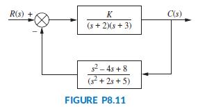
For the system shown in Figure P8.11, do the following:a. Sketch the root locus.b. Find the jω-axis crossing and the gain, K, at the crossing.c. Find the real-axis breakaway to two-decimal-place
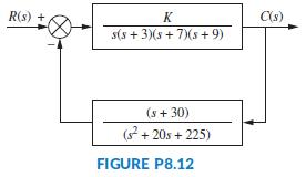
Sketch the root locus for the system of Figure P8.12 and find the following:a. The range of gain to yield stabilityb. The value of gain that will yield a damping ratio of 0.707 for the system’s
Repeat Problem 39 using MATLAB. The program will do the following in one program:a. Display a root locus and pause.b. Display a close-up of the root locus where the axes go from -2 to 0.5 on the real
Given the unity feedback system shown in Figure P8.3 where do the following:a. If z = 2, find K so that the damped frequency of oscillation of the transient response is 5 rad/s.b. For the system of
Given the unity feedback system shown in Figure P8.3, wherefind the following:a. The value of gain, K, that will yield a settling time of 4 secondsb. The value of gain, K, that will yield a
You are given the unity-feedback system of Figure P8.3, whereUse MATLAB to plot the root locus. Use a closeup of the locus (from -5 to 0 and — 1 to 6) to find the gain, K, that yields a closed-loop
Letin Figure P8.3.a. Find the range of K for closed-loop stability.b. Plot the root locus for K > 0.c. Plot the root locus for K < 0.d. Assuming a step input, what value of K will result in the
Given the unity feedback system shown in Figure P8.3, whereevaluate the pole sensitivity of the closed-loop system if the second-order, underdamped closed-loop poles are set fora. ζ = 0:591b. ζ =
Repeat Problem 3 but sketch your root loci for negative values of K.Data From Problem 3:Sketch the root locus for the unity feedback system shown in Figure P8.3for the following transfer
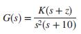
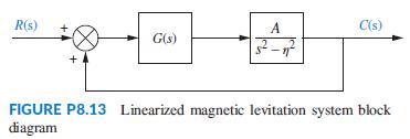
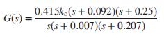
Figure P8.13 shows the block diagram of a closed loop control of a linearized magnetic levitation system (Galvão, 2003)..Assuming A = 1300 and η = 860, draw the root locus and find the range of K
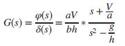
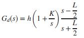
The simplified transfer function model from steering angle δ(s) to tilt angle φ(s) in a bicycle is given byIn this model, h represents the vertical distance from the center of mass to the floor, so
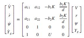
A technique to control the steering of a vehicle that follows a line located in the middle of a lane is to define a look-ahead point and measure vehicle deviations with respect to the point. A
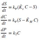
It is known that mammals have hormonal regulation mechanisms that help maintain almost constant calcium plasma levels (0.08–0.1 g/L in dairy cows). This control is necessary to maintain healthy
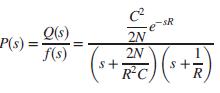
Problem 64 in Chapter 7 introduced the model of a TCP/IP router whose packet-drop probability is controlled by using a random early detection (RED) algorithm (Hollot, 2001). Using Figure P8.3 as a
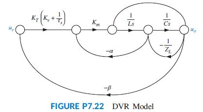
For the dynamic voltage restorer (DVR) discussed in Problem 47, Chapter 7, do the following:a. When ZL = 1/sCL, a pure capacitance, the system is more inclined toward instability. Find the system’s
The closed-loop vehicle response in stopping a train depends on the train’s dynamics and the driver, who is an integral part of the feedback loop. In Figure P8.3, let the input be R(s) = vr the
Voltage droop control is a technique in which loads are driven at lower voltages than those provided by the source. In general, the voltage is decreased as current demand increases in the load. The
It has been suggested that the use of closed-loop feedback in ventilators can highly reduce mortality and health problems in patients in need of respiratory treatments (Hahn, 2012). A good knowledge
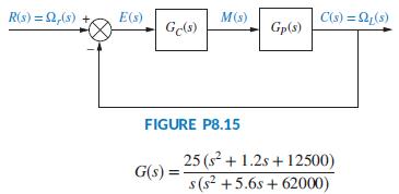
Figure P8.15 shows a simplified drawing of a feedback system that includes the drive systempresented in Problem 67, Chapter 5 (Thomsen, 2011). Referring to Figures P5.43 and P8.15, Gp(s) in Figure
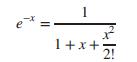
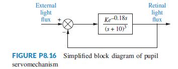
A simplified block diagram of a human pupil servomechanism is shown in Figure P8.16. The term e -0.18s represents a time delay. This function can be approximated by what is known as a Padé
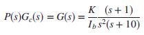
A hard disk drive (HDD) arm has an open-loop unstable transfer function,where X(s) is arm displacement and F(s) is the applied force (Yan, 2003). Assume the arm has an inertia of Ib = 3 × 10-5 kg-m2
A robotic manipulator together with a cascade PI controller has a transfer function (Low, 2005)Assume the robot’s joint will be controlled in the configuration shown in Figure P8.3.a. Find the
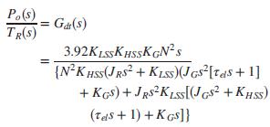
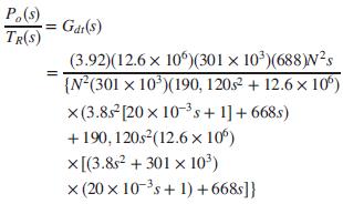
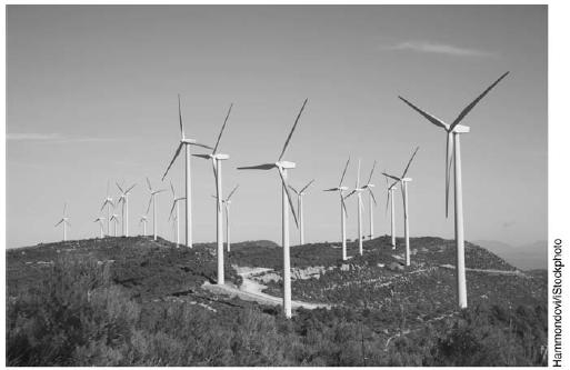
Wind turbines, such as the one shown in Figure P8.17(a), are becoming popular as a way of generating electricity. Feedback control loops are designed to control the output power of the turbine, given
An active system for the elimination of floor vibrations due to human presence is presented in (Nyawako, 2009). The system consists of a sensor that measures the floor’s vertical acceleration and
Many implantable medical devices such as pacemakers, retinal implants, deep brain stimulators, and spinal cord stimulators are powered by an in-body battery that can be charged through a
It is important to precisely control the amount of organic fertilizer applied to a specific crop area in order to provide specific nutrient quantities and to avoid unnecessary environmental
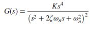
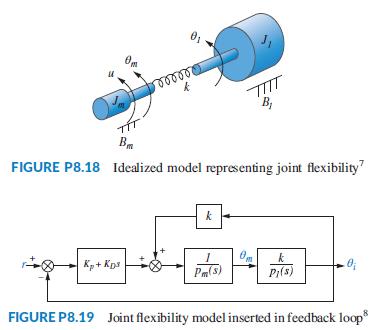
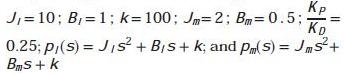
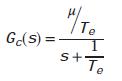
Harmonic drives are very popular for use in robotic manipulators due to their low backlash, high torque transmission, and compact size (Spong, 2006). The problem of joint flexibility is sometimes a
Using LabVIEW, the Control Design and Simulation Module, and the Math Script RT Module, open and customize the Interactive Root Locus VI from the Examples to implement the system of Problem 64.
An automatic regulator is used to control the field current of a three phase synchronous machine with identical symmetrical armature windings (Stapleton,1964). The purpose of the regulator is to
It is well known that when a person ingests a significant amount of water, the blood volume increases, causing an increase in arterial blood pressure until the kidneys are able to excrete the excess
One of the treatments for Parkinson’s disease in some patients is Deep Brain Stimulation (DBS) (Davidson, 2012). In DBS a set of electrodes is surgically implanted and a vibrating current is
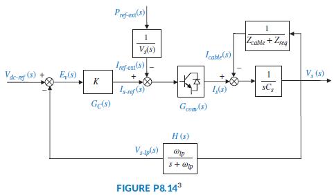
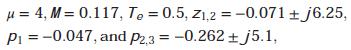
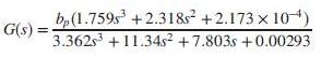
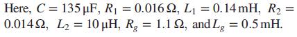
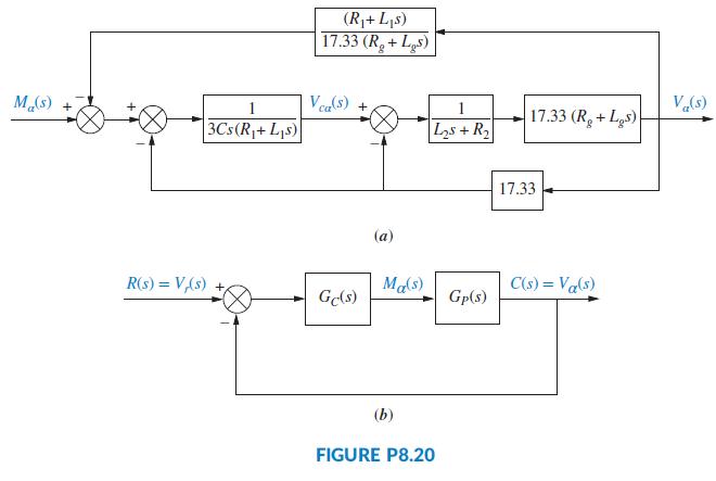
A linear dynamic model of the α-subsystem of a grid connected voltage source converter (VSC) using a Y-Y transformer is shown in Figure P8.20 (a) (Mahmood, 2012).a. Find the transfer function GP(s)
Consider the fluid temperature control of a parabolic trough collector (Camocho, 2012) embedded in the unity feedback structure as shown in Figure P8.3, where the open-loop plant transfer function is
Define the transfer function.
What transformation turns the solution of differential equations into algebraic manipulations?
What mathematical model permits easy interconnection of physical systems?
Briefly describe each of your answers to Question 15.Data From Question 15:Name three approaches to the mathematical modeling of control systems.
Name three approaches to the mathematical modeling of control systems.
Adjustments of the forward path gain can cause changes in the transient response. True or false?
Describe a typical control system design task.

Showing 800 - 900 of 943