New Semester Started Get 50% OFF Study Help! --h --m --s Claim Now

Question Answers

Textbooks

Find textbooks, questions and answers

Oops, something went wrong!

Change your search query and then try again

Result Not Found

Books FREE
Study Help
Tutors
AI Study Planner NEW
Sell Books

Search
Sign In
Register

study help
engineering
control systems engineering

Control Systems Engineering 7th Edition Norman S. Nise - Solutions

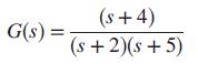
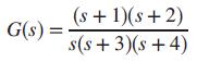
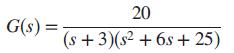
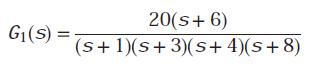
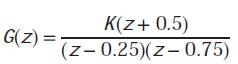
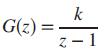
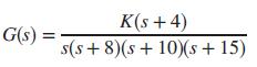
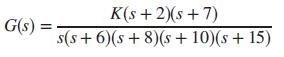
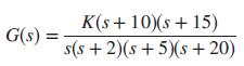
Using partial-fraction expansion and Table 13.1, find the z-transform for each G(s) shown below if T = 0.5 second.a.b.c.d.Data from Table 13.1 (s+4) G(s) = (s +2)(s + 5)
Name two methods of finding the inverse z-transform.
Repeat all parts of Problem 6 using MATLAB and MATLAB’s Symbolic Math Toolbox.Data from Problem 6Using partial-fraction expansion and Table 13.1, find the z-transform for each G(s) shown below if T = 0.5 second.a.b.c.d.Data from Table 13.1 (s+4) G(s) = (s +2)(s + 5)
What method for finding the inverse z-transform yields a closed-form expression for the time function?
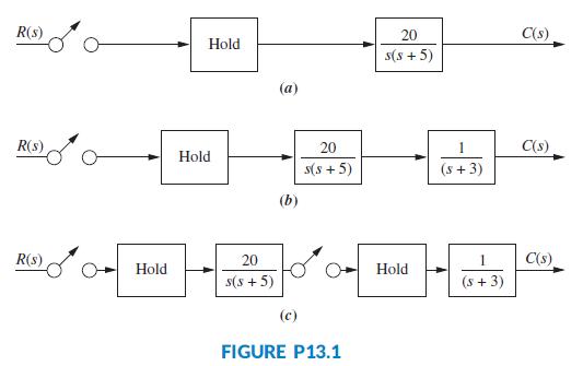
Find G(z) = C(z)/R(z) for each of the block diagrams shown in Figure P13.1 if T = 0.3 second. R(s) 20 C(s) Hold s(s + 5) (a) R(s) 20 C(s) Hold s(s + 5) (s + 3) (b) R(s) 20 C(s) Hold Hold s(s + 5) (s + 3) (c) FIGURE P13.1
What method for finding the inverse z-transform immediately yields the values of the time waveform at the sampling instants?
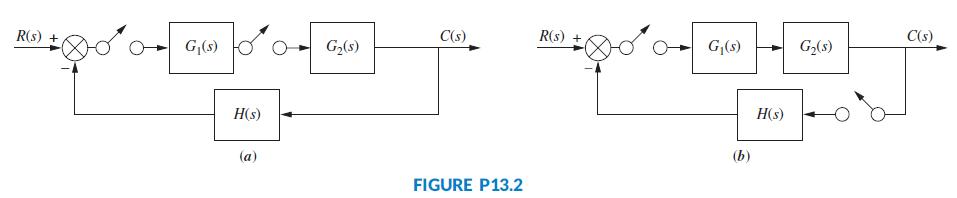
Find T(z) = C(z)/R(z) for each of the systems shown in Figure P13.2. R(s) + C(s) R(s) C(s) + G,(s) G,(s) G(s) G2(s) H(s) H(s) (a) (b) FIGURE P13.2
In order to find the z-transform of a G(s), what must be true of the input and the output?
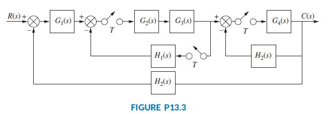
Find C(z) in general terms for the digital system shown in Figure P13.3. R(s) +, C(s) G,(s) O- G,(s) G3(3) GĄ(s) T T H (s) H,(s) T H,(s) FIGURE P13.3
If input R(z) to system G(z) yields output C(z), what is the nature of c(t)?
If a time waveform, c(t), at the output of system G(z) is plotted using the inverse z-transform, and a typical second-order response with damping ratio = 0.5 results, can we say that the system is stable?
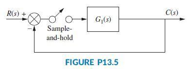
Write a MATLAB program that can be used to find the range of sampling time, T, for stability. The program will be used for systems of the type represented in Figure P13.5 and should meet the following requirements:a. MATLAB will convert G1(s) cascaded with a sample-and-hold to G(z).b. The program
What must exist in order for cascaded sampled-data systems to be represented by the product of their pulse transfer functions, G(z)?
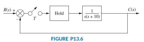
Given the system in Figure P13.6, find the range of sampling interval, T, that will keep the system stable. C(s) R(s) + Hold s(s + 10) FIGURE P13.6
Where is the region for stability on the z-plane?
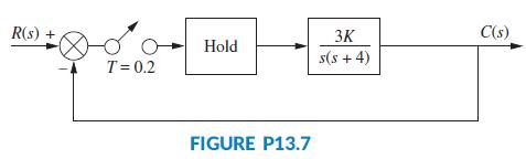
Find the range of gain, K, to make the system shown in Figure P13.7 stable. R(s) + 3K C(s) Hold s(s + 4) T= 0.2 FIGURE P13.7
What methods for finding the stability of digital systems can replace the Routh-Hurwitz criterion for analog systems?
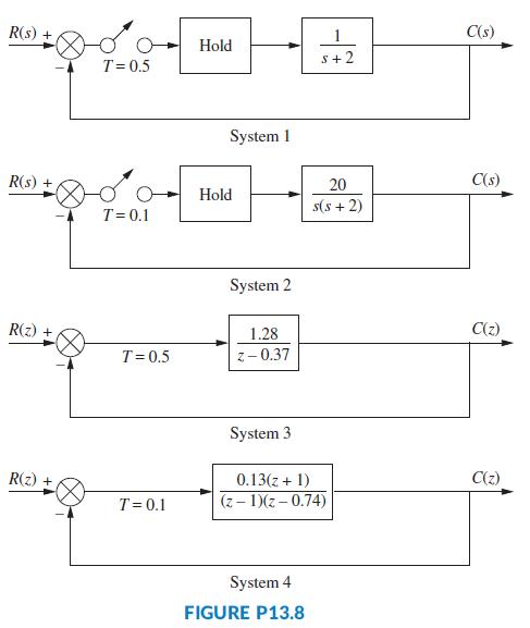
Find the static error constants and the steady-state error for each of the digital systems shown in Figure P13.8 if the inputs area. u (t)b. t u(t)c. 1/2 t2 u(t) R(s) + 1 C(s) Hold S+ 2 T= 0.5 System 1 R(s) 20 C(s) O- Hold s(s + 2) T= 0.1 System 2 R(z) + 1.28 C(z) T= 0.5 z-0.37 System 3 R(z) +
To drive steady-state errors in analog systems to zero, a pole can be placed at the origin of the s-plane. Where on the z-plane should a pole be placed to drive the steady-state error of a sampled system to zero?
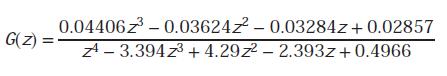
Write a MATLAB program that can be used to find Kp, Kv, and Ka for digital systems. The program will be used for systems of the type represented in Figure P13.5. Test your program forwhere G(z) is the pulse transfer function for G1(s) in cascade with the z.o.h. and T = 0.1 second.
How do the rules for sketching the root locus on the z-plane differ from those for sketching the root locus on the s-plane?
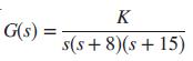
For the digital system shown in Figure P13.5, where G1(s) = K/[(s + 1)(s + 5)], find the value of K to yield a 15% overshoot. Also find the range of K for stability. Let T = 0.1 second. C(s) R(s) +
Given a point on the z-plane, how can one determine the associated percent overshoot, settling time, and peak time?
Given a desired percent overshoot and settling time, how can one tell which point on the z-plane is the design point?
For the digital system shown in Figure P13.5, where G1(s) = K(s + 2) ÷ [s(s + 1)(s + 3)], find the value of K to yield a settling time of 15 seconds if the sampling interval, T, is 1 second. Also, find the range of K for stability.
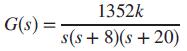
Repeat Problem 25 using MATLAB. Data from Problem 25A continuous unity feedback system has a forward transfer function ofThe system is to be computer controlled with the following specifications: Percent overshoot: 10% Settling time: 2 seconds Sampling interval: 0:01
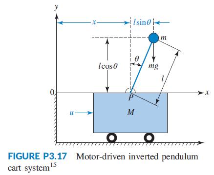
An inverted pendulum mounted on a motor-driven cart (Prasad, 2012) was the subject of Problem 33, Chapter 9. In that problem you were asked to develop Simulink models for two feed back systems, one of which was to control the cart position, x(t). At the recommended settings, the step response of
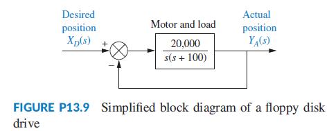
The analog system of a disk drive is shown in Figure P13.9. Do the following:a. Convert the disk drive to a digital system. Use a sampling time of 0.01 second.b. Find the range of digital controller gain to keep the system stable.c. Find the value of digital controller gain to yield 15% overshoot
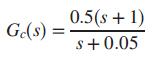
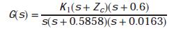
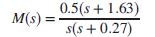
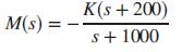
In Problem 49, Chapter 9, and Problem 39, Chapter 10, we considered the radial pickup position control of a DVD player. A controller was designed and placed in cascade with the plant in a unit feedback configuration to stabilize the system. The controller was given byand the plant by (Bittanti,
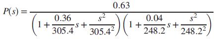
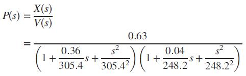
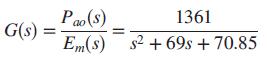
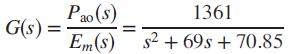
In Problem 24, Chapter 11, we discussed an EVAD, a device that works in parallel with the human heart to help pump blood in patients with cardiac conditions. The device has a transfer functionwhere Em(s) is the motor’s armature voltage, and Pao(s) is the aortic blood pressure (Tasch, 1990). Using
In Problem 47, Chapter 9, a steam-driven turbine governor system was implemented by a unity feedback system with a forward-path transfer function (Khodabakhshian, 2005)a. Use a sampling period of T = 0.5 s and find a discrete equivalent for this system.b. Use MATLAB to draw the root locus.c. Find
Discrete time controlled systems can exhibit unique characteristics not available in continuous controllers. For example, assuming a specific input and some conditions, it is possible to design a system to achieve steady state within one single time sample without overshoot. This scheme is well
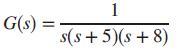
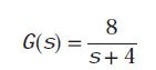
GivenUse the LabVIEW Control Design and Simulation Module to (1) convert G(s) to a digital transfer function using a sampling rate of 0.25 second; and (2) plot the step responses of the discrete and the continuous transfer functions. 8 G(s) = S+4
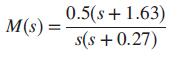
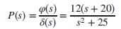
GivenUse the LabVIEW Control Design and Simulation Module and the Math Script RT Module to (1) obtain the value of K that will yield a damping ratio of 0.5 for the closed loop system in Figure 13.20, where H(z)=1; and (2) display the step response of the closed-loop system in Figure 13.20 where
Obtaining an exact shape in metal forming can be tricky because of material spring back. A feedback system has been devised in which critical deviations from specifications are measured as soon as a part is formed and automatic incremental corrections to the forming tools are made before the next
The purpose of an artificial pacemaker is to regulate heart rate in those patients in which the natural feedback system malfunctions. Assume a unity-feedback system with a forward path,as a simplified model of a pacemaker (Neogi, 2010).a. Convert the pacemaker model to a discrete system with a
A linear model of the α-subsystem of a grid-connected voltage-source converter with a Y-Y transformer (Mahmood, 2012) was presented in Problem 69, Chapter 8, and Problem 51, Chapter 10. The system was represented with unity-feedback and a forward path consisting of the cascading of a compensator
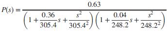
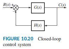
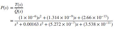
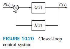
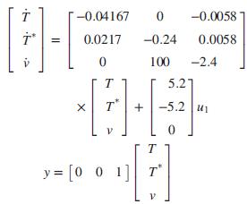
The linearized model for an HIV/AIDS patient treated with RTIs was obtained in Chapter 6 as (Craig, 2004);a. Consider this plant in the feedback configuration in Figure 10.20 with G(s) = P(s) and H(s) = 1. Obtain the Nyquist diagram. Evaluate the system for closed loop stability.b. Consider this
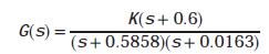
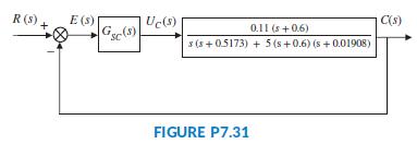
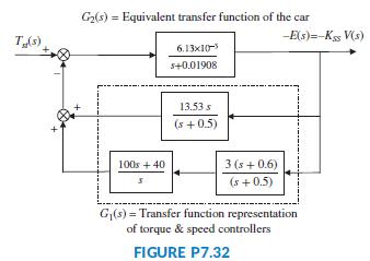
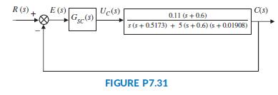
In Problem 71, Chapter 8, we used MATLAB to plot the root locus for the speed control of an HEV rearranged as a unity-feedback system, as shown in Figure P7.31 (Preitl, 2007). The plant and compensator were given byand we found that K = 0.78, resulted in a critically damped system.a. Use MATLAB or
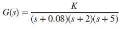
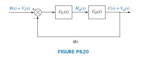
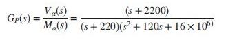
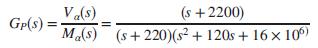
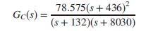
A linear model of the α-subsystem of a grid connected voltage-source converter (VSC) with a Y-Y transformer (Mahmood, 2012) was presented in Problem 69, Chapter 8. In Figure P8.20(b), GC(s) = K and GP(s) is given in a pole zero form (with a unity gain and slightly modified parameters) as
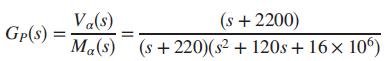
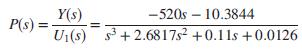
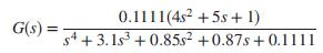
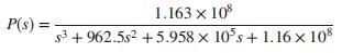
A new measurement-based technique to design fixed structure controllers for unknown SISO systems, which does not require system identification, has been proposed. The fourth-order transfer function shown below and modified to have a unity steady state gain is used as an example (Khadraoui,
What major advantage does compensator design by frequency response have over root locus design?
How is gain adjustment related to the transient response on the Bode diagrams?
For each of the systems in Problem1, design the gain, K, for a phase margin of 40°.
Briefly explain how a lag network allows the low-frequency gain to be increased to improve steady-state error without having the system become unstable.
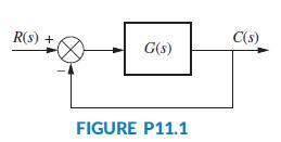
Given the unity feedback system of Figure P11.1, use frequency response methods to determine the value of gain, K, to yield a step response with a 20% overshoot ifa.b.c.
From the Bode plot perspective, briefly explain how the lag network does not appreciably affect the speed of the transient response.
Given the unity feedback system of Figure P11.1 withdo the following:a. Use frequency response methods to determine the value of gain, K, to yield a step response with a 20% overshoot. Make any required second-order approximations.b. Use MATLAB or any other computer program to test your second
Modify the MATLAB program you developed in Problem 10.20 to do the following:a. Display the closed-loop magnitude and phase frequency response plots for the drive system(Thomsen,2011)presented in Problem 56, Chapter 8. Using the graph properties, specify the value of K in the Bode plot
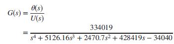
In order to self-balance a bicycle, its open-loop transfer function is found to be (Lam, 2011):where θ(s) is the angle of the bicycle with respect to the vertical, and U(s) is the voltage applied to the motor that drives a flywheel used to stabilize the bicycle. Note that the bicycle is open-loop
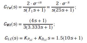
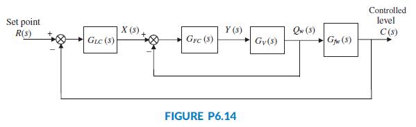
The block diagram of a cascade system used to control water level in a steam generator of a nuclear power plant (Wang, 2009) was presented in FigureP6.14. In that system, the level controller, GLC(s), is the master controller and the feed-water flow controller, GFC(s), is the slave controller.
Use LabVIEW with the Control Design and Simulation Module, and Math Script RT Module to build a VI that will accept an open-loop transfer function, plot the Bode diagram, and plot the closed-loop step response. Your VI will also use the CD Parametric Time Response VI to display (1) rise time, (2)
Use LabVIEW with the Control Design and Simulation Module and MathScript RT Module to do the following: Modify the CDEx Nyquist Analysis.vi to obtain the range of K for stability using the Nyquist plot for any system you enter. In addition, design a LabVIEW VI that will accept as an input the
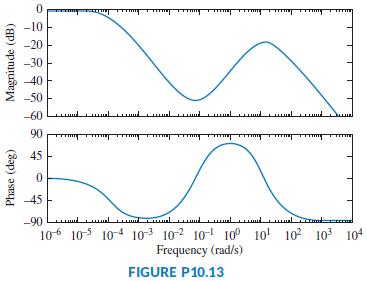
The design of cruise control systems in heavy vehicles, such as big rigs, is especially challenging due to the extreme variations in payload. Assume that the frequency response for the transfer function from fuel mass flow to vehicle speed is shown in Figure P10.13.This response includes the
An experimental holographic media storage system uses a flexible photopolymer disk. During rotation, the disk tilts, making information retrieval difficult. A system that compensates for the tilt has been developed. For this, a laser beam is focused on the disk surface and disk variations are
In the TCP/IP network link of Problem 41, let L = 0.8, but assume that the amount of delay is an unknown variable.a. Plot the Nyquist diagram of the system for zero delay, and obtain the phase margin.b. Find the maximum delay allowed for closed-loop stability.
The linearized model of a particular network link working under TCP/IP and controlled using a random early detection (RED) algorithm can be described by Figure 10.20 where G(s) = M(s)P(s); H = 1, and (Hollot, 2001)a. Plot the Nichols chart for L = 1. Is the system closed-loop stable?b. Find the
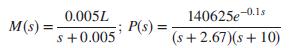
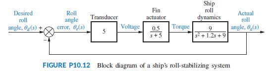
A ship’s roll can be stabilized with a control system. A voltage applied to the fins’ actuators creates a roll torque that is applied to the ship. The ship, in response to the roll torque, yields a roll angle. Assuming the block diagram for the roll control system shown in Figure P10.12,
The control of the radial pickup position of a digital versatile disk (DVD) was discussed in Problem 48, Chapter 9. There, the open-loop transfer function from coil input voltage to radial pickup position was given asAssume the plant is in cascade with a controller,and in the closed-loop
A simple modified and linearized model for the transfer function of a certain bicycle from steer angle (δ) to roll angle (φ) is given by (Åstrom, 2005)Assume the rider can be represented by a gain K, and that the closed-loop system is shown in Figure 10.20 with G(s)= KP(s) and H = 1. Use
Problem 47, Chapter 8 discusses a magnetic levitation system with a plant transfer function P(s) = 1300/s2 - 8602 (Galvão, 2003). Assume that the plant is in cascade with an M(s) and that the system will be controlled by the loop shown in Figure 10.20, where G(s) = M(s)P(s) and H = 1. For
A room’s temperature can be controlled by varying the radiator power. In a specific room, the transfer function from in door radiator power, Q, to room temperature, T in °C is (Thomas, 2005)The system is controlled in the closed-loop configuration shown in Figure 10.20 with G(s) = KP(s); H =
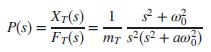
An overhead crane consists of a horizontally moving trolley of mass mT dragging a load of mass mL, which dangles from its bottom surface at the end of a rope of fixed length, L. The position of the trolley is controlled in the feedback configuration shown in Figure 10.20. Here, G(s) = KP(s); H = 1,
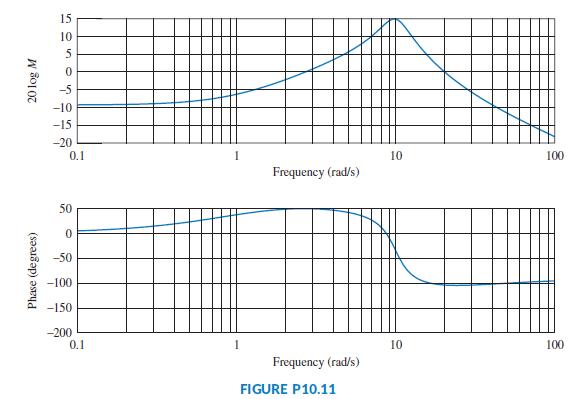
Repeat Problem 32 for the Bode plots shown in Figure P10.11. 15 10 5 -5 -10 -15 -20 0.1 10 100 Frequency (rad/s) 50 -50 -100 -150 -200 0.1 10 100 Frequency (rad/s) FIGURE P10.11 Phase (degrees) 20 log M
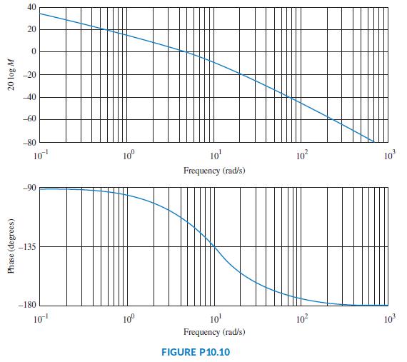
For the Bode plots shown in Figure P10.10, determine the transfer function by hand or via MATLAB. 40 20 -20 -40 -60 -80 10 10° 10' 10 10 Frequency (rad/s) -90 -135 -180 10 10° 10' 10? 10 Frequency (rad/s) FIGURE P10.10 Phase (degrees) 20 log M
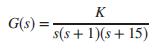
Given a unity feedback system with the forward-path transfer functionand a delay of 0.2 second, make a second-order approximation and estimate the percent overshoot if K = 30. Use Bode plots and frequency response techniques. K G(s) s(s + 1)(s+ 15)
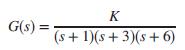
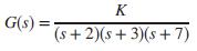
Given a unity feedback system with the forward-path transfer functionand a delay of 0.5 second, find the range of gain, K, to yield stability. Use Bode plots and frequency response techniques. K G(s) = (s + 1)(s+ 3)(s+6)
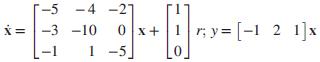
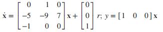
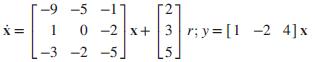
For each of the following closed-loop systems, find the steady-state error for unit step and unit ramp inputs. Use both the final value theorem and input substitution methods.a.b.c. -5 -4 -21 X = -3 -10 0 x+1 r; y = [-1 2 1]x - 1 -5]
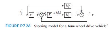
A simplified model of the steering of a four-wheel drive vehicle is shown in Figure P7.26.In this block diagram, the output r is the vehicle’s yaw rate, while δf and δr are the steering angles of the front and rear tires, respectively. In this model,and K(s) is a controller to be designed.
Glycolysis is a feedback process through which living cells use glucose to generate adenosine triphosphate (ATP), necessary for cell operations. A linearized glycolysis model (Chandra, 2011) is given bywhere δ is the perturbation (disturbance input) on ATP production, Δy is the change in ATP
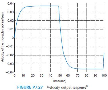
As part of the development of a textile cross-lapper machine (Kuo, 2010), a torque input,is applied to the motor of one of the movable racks embedded in a feedback loop. The corresponding velocity output response is shown in Figure P7.27.a. What is the open-loop system’s type?b. What is the
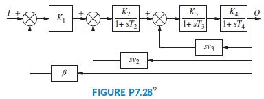
The block diagram in Figure P7.28 represents a motor driven by an amplifier with double-nested tachometer feedback loops (Mitchell, 2010).a. Find the steady-state error of this system to a step input.b. What is the system type? K2 1+ sT, K3 1+ sT K4 1+ sT SV3 SV2 FIGURE P7.28° 04
A Type 3 feedback control system (Papadopoulos, 2013) was presented in Problem 60. Modify the Simulink model you developed in that problem to plot its response (from 0 to 100 seconds) to a unit-ramp reference input, r(t) = tu(t), applied at t = 0, and (on the same graph) to a disturbance, d(t) =
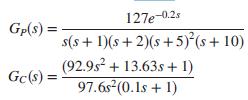
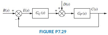
PID control, may be recommended for Type 3 systems when the output in a feedback system is required to perfectly track a parabolic as well as step and ramp reference signals (Papadopoulos, 2013). In the system of Figure P7.29, the transfer functions of the plant, GP(s), and the recommended
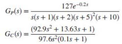
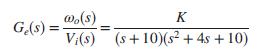
An open-loop swivel controller and plant for an industrial robot has the transfer functionwhere ωo(s) is the Laplace transform of the robot’s angular swivel velocity and Vi(s) is the input voltage to the controller. Assume Ge(s) is the forward transfer function of a velocity control loop with an
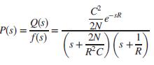
Packet information flow in a router working under TCP/IP can be modeled using the linearized transfer functionwhereC = link capacity (packets/second)N = load factor (number of TCP sessions)Q= expected queue lengthR = round trip time (second)p =probability of a packet dropThe objective of an active
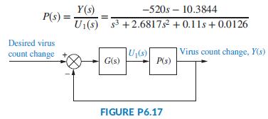
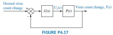
Consider the HIV infection model of Problem 68 in Chapter 6 and its block diagram in Figure P6.17 (Craig, 2004).a. Find the system’s type if G(s) is a constant.b. It was shown in Problem 68, Chapter 6, that when G(s) = K the system will be stable when K < 2.04 × 10-4. What value of K will
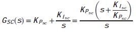
Figure P7.31 shows the block diagram of the speed control of an HEV taken from Figure P5.53, and rearranged as a unity feedback system (Preitl, 2007). Here the system output is C(s) = KSSV(s), the output voltage of the speed sensor/transducer.a. Assume the speed controller is given as GSC(s) = KPSC
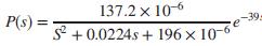
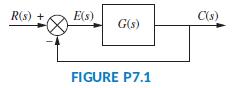
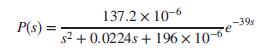
The parabolic trough collector (Camacho, 2012) is embedded in a unit feedback configuration as shown in Figure P7.1, where G(s) = GC(s)P(s) anda. Assuming GC(s) = K, find the value of K required for a unit-step input steady-state error of 3%. Use the result you obtained in Problem 70, Chapter 6, to
What is a root locus?
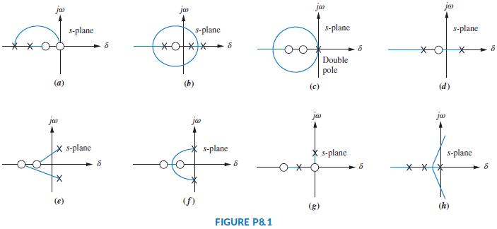
For each of the root loci shown in Figure P8.1, tell whether or not the sketch can be a root locus. If the sketch cannot be a root locus, explain why. Give all reasons. jo ja ja ja s-plane s-plane s-plane s-plane Double pole (b) (c) (d) ja ja ja ja X s-plane s-plane * s-plane s-plane *** (e) (g)
Describe two ways of obtaining the root locus.
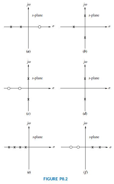
Sketch the general shape of the root locus for each of the open-loop pole-zero plots shown in Figure P8.2. ja ja s-plane s-plane (a) (b) ja ja s-plane s-plane (c) (d) ja ja splane splane *** ** FIGURE P8.2
If KG(s)H(s) = 5 < 180°, for what value of gain is s a point on the root locus?
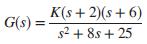
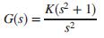
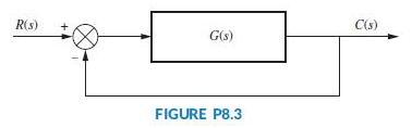
Sketch the root locus for the unity feedback system shown in Figure P8.3for the following transfer functions:a.b.c.d. K(s + 2)(s + 6) s2 + 8s + 25 G(s) =
Do the zeros of a system change with a change in gain?
Where are the zeros of the closed-loop transfer function?
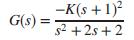
Letwith K > 0 in Figure P8.3.a. Find the range of K for closed-loop stability.b. Sketch the system’s root locus.c. Find the position of the closed-loop poles when K = 1 and K = 2. -K(s + 1)? G(s): s2 +2s + 2
What are two ways to find where the root locus crosses the imaginary axis?
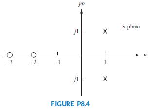
For the open-loop pole-zero plot shown in Figure P8.4, sketch the root locus and find the break-in point. ja s-plane jl -3 -2 -1 -jl FIGURE P8.4
How can you tell from the root locus if a system is unstable?
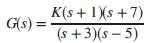
Sketch the root locus of the unity feedback system shown in Figure P8.3, whereand find the break-in and breakaway points. Find the range of K for which the system is closed-loop stable. K(s + 1)s +7) G(s) (s +3)(s - 5) %3D
In the linearized model of Chapter 6, Problem68, where virus levels are controlled by means of RTIs, the open-loop plant transfer function was shown to beThe amount of RTIs delivered to the patient will automatically be calculated by embedding the patient in the control loop as G(s) shown in Figure
In Chapter 7, Figure P7.31 shows the block diagram of the speed control of an HEV rearranged as a unity feedback system (Preitl, 2007). Let the transfer function of the speed controller bea. Assume first that the speed controller is configured as a proportional controller KISC = 0 and GSC (s) =
Briefly distinguish between the design techniques in Chapter 8 and Chapter 9.
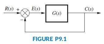
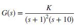
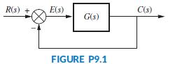
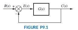
Design a PI controller to drive the step response error to zero for the unity feedback system shown in Figure P9.1, whereThe system operates with a damping ratio of 0.6. Compare the specifications of the uncompensated and compensated systems. K G(s) = (s+ 1) (s+ 10)
Name two major advantages of the design techniques of Chapter 9 over the design techniques of Chapter 8.
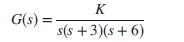
Consider the unity feedback system shown in Figure P9.1, wherea. Design a PI controller to drive the ramp response error to zero for any K that yields stability.b. Use MATLAB to simulate your design for K = 1. Show both the input ramp and the output response on the same plot. K G(s) = s(s +3)(s+ 6)
What kind of compensation improves the steady-state error?
The unity feedback system shown in Figure P9.1 withis operating with 10% overshoot.a. What is the value of the appropriate static error constant?b. Find the transfer function of a lag network so that the appropriate static error constant equals 4 without appreciably changing the dominant poles of

Showing 200 - 300 of 942

1
2
3
4
5
6
7
8
9
10

Step by Step Answers

Services

Sitemap
Fun
Definitions
Become Tutor
Used Textbooks
Study Help Categories
Recent Questions
Expert Questions
Campus Wear
Sell Your Books

Company Info

Security
Copyrights
Privacy Policy
Terms & Conditions
SolutionInn Fee
Scholarship
Online Quiz
Give Feedback, Get Rewards

Get In Touch

About Us
Contact Us
Career
Jobs
FAQ
Student Discount
Campus Ambassador

Secure Payment

Download Our App

© 2026 SolutionInn. All Rights Reserved