New Semester Started Get 50% OFF Study Help! --h --m --s Claim Now

Question Answers

Textbooks

Find textbooks, questions and answers

Oops, something went wrong!

Change your search query and then try again

Result Not Found

Books FREE
Study Help
Tutors
AI Study Planner NEW
Sell Books

Search
Sign In
Register

study help
engineering
control systems engineering

Control Systems Engineering 7th Edition Norman S. Nise - Solutions

What kind of compensation improves transient response?
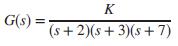
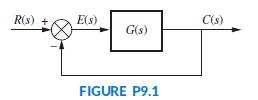
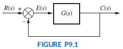
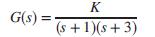
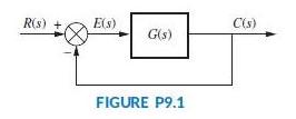
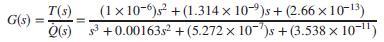
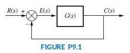
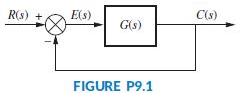
Repeat Problem 3 for G(s) = K/s(s + 3)(s + 7).Data from Problem 3:The unity feedback system shown in Figure P9.1 withis operating with 10% overshoot.a. What is the value of the appropriate static error constant?b. Find the transfer function of a lag network so that the appropriate static error
What kind of compensation improves both steady-state error and transient response?
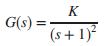
Consider the unity feedback system shown in Figure P9.1 witha. Design a compensator that will yield Kp = 20 without appreciably changing the dominant pole location that yields a 10% overshoot for the uncompensated system.b. Use MATLAB or any other computer program to simulate the uncompensated and
Cascade compensation to improve the steady-state error is based upon what pole-zero placement of the compensator? Also, state the reasons for this placement.
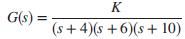
The unity feedback system shown in Figure P9.1 withis operating with a dominant-pole damping ratio of 0.707. Design a PD controller so that the settling time is reduced by a factor of 2. Compare the transient and steady-state performance of the uncompensated and compensated systems. Describe any
Cascade compensation to improve the transient response is based upon what pole-zero placement of the compensator? Also, state the reasons for this placement.
Redo Problem 6 using MATLAB in the following way:a. MATLAB will generate the root locus for the uncompensated system along with the 0.707 damping ratio line. You will interactively select the operating point. MATLAB will then inform you of the coordinates of the operating point, the gain at the
What difference on the s-plane is noted between using a PD controller or using a lead network to improve the transient response?
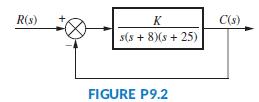
Design a PD controller for the system shown in Figure P9.2 to reduce the settling time by a factor of 4 while continuing to operate the system with 20.5% overshoot. Compare the performance of the compensated system to that of the uncompensated system. Summarize the results in a table similar to
In order to speed up a system without changing the percent overshoot, where must the compensated system’s poles on the s-plane be located in comparison to the uncompensated system’s poles?
Consider the unity feedback system shown in Figure P9.1 with a. Find the location of the dominant poles to yield a 1.2 second settling time and an overshoot of 15%.b. If a compensator with a zero at -1 is used to achieve the conditions of Part a, what must the angular contribution of the
Why is there more improvement in steady-state error if a PI controller is used instead of a lag network?
The unity feedback system shown in Figure P9.1 with G(s) = K/s2 is to be designed for a settling time of 1.667 seconds and a 16.3% overshoot. If the compensator zero is placed at -1, do the following:a. Find the coordinates of the dominant poles.b. Find the compensator pole.c. Find the system
When compensating for steady-state error, what effect is sometimes noted in the transient response?
Given the unity feedback system of Figure P9.1, withdo the following:a. Sketch the root locus.b. Find the coordinates of the dominant poles for which ζ = 0.8.c. Find the gain for which ζ = 0.8.d. If the system is to be cascade-compensated so that Ts = 1 second and ζ = 0.8, find the compensator
A lag compensator with the zero 25 times as far from the imaginary axis as the compensator pole will yield approximately how much improvement in steady-state error?
Redo Problem 11 using MATLAB in the following way:a. MATLAB will generate the root locus for the uncompensated system along with the 0.8 damping ratio line. You will interactively select the operating point. MATLAB will then inform you of the coordinates of the operating point, the gain at the
If the zero of a feedback compensator is at -3 and a closed-loop system pole is at -3.001, can you say there will be pole-zero cancellation? Why?
Consider the unity feedback system of Figure P9.1 withThe system is operating at 20% overshoot. Design a compensator to decrease the settling time by a factor of 2 without affecting the percent overshoot and do the following:a. Evaluate the uncompensated system’s dominant poles, gain, and
Name two advantages of feedback compensation.
The unity feedback system shown in Figure P9.1 withis operating with 30% overshoot.a. Find the transfer function of a cascade compensator, the system gain, and the dominant pole location that will cut the settling time in half if the compensator zero is at -7.b. Find other poles and zeros and
For the unity feedback system of Figure P9.1 withdo the following:a. Find the settling time for the system if it is operating with 15% overshoot.b. Find the zero of a compensator and the gain, K, so that the settling time is 7 seconds. Assume that the pole of the compensator is located at =15.c.
A unity feedback control system has the following forward transfer function:a. Design a lead compensator to yield a closed-loop step response with 20.5% overshoot and a settling time of 3 seconds. Be sure to specify the value of K.b. Is your second-order approximation valid?c. Use MATLAB or any
For the unity feedback system of Figure P9.1, withthe damping ratio for the dominant poles is to be 0.4, and the settling time is to be 0.5 second.a. Find the coordinates of the dominant poles.b. Find the location of the compensator zero if the compensator pole is at -15.c. Find the required system
Consider the unity feedback system of Figure P9.1, witha. Show that the system cannot operate with a settling time of 2/3 second and a percent overshoot of 1.5 % with a simple gain adjustment.b. Design a lead compensator so that the system meets the transient response characteristics of Part a.
Given the unity feedback system of Figure P9.1 withFind the transfer function of a lag-lead compensator that will yield a settling time 0.5 second shorter than that of the uncompensated system. The compensated system also will have a damping ratio of 0.5, and improve the steady-state error by a
Redo Problem 19 using a lag-lead compensator and MATLAB in the following way:a. MATLAB will generate the root locus for the uncompensated system along with the 0.5 damping-ratio line. You will interactively select the operating point. MATLAB will then proceed to inform you of the coordinates of the
Given the uncompensated unity feedback system of Figure P9.1, withdo the following:a. Design a compensator to yield the following specifications: settling time = 2.86 seconds; percent overshoot = 4.32%; the steady-state error is to be improved by a factor of 2 over the uncompensated system.b.
For the unity feedback system given in Figure P9.1 withdo the following:a. Find the gain, K, for the uncompensated system to operate with 30% overshoot.b. Find the peak time and Kv for the uncompensated system.c. Design a lag-lead compensator to decrease the peak time by a factor of 2, decrease the
The unity feedback system shown in Figure P9.1 withis to be designed to meet the following specifications:Overshoot: Less than 22%Settling time: Less than 1.6 secondsKp = 15Do the following:a. Evaluate the performance of the uncompensated system operating at approximately 10% overshoot.b. Design a
Consider the unity feedback system in Figure P9.1, withThe system is operated with 4.32% overshoot. In order to improve the steady-state error, Kp is to be increased by at least a factor of 5. A lag compensator of the formis to be used.a. Find the gain required for both the compensated and the
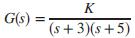
For the unity feedback system in Figure P9.1, withdesign a PID controller that will yield a peak time of 1.122 seconds and a damping ratio of 0.707, with zero error for a step input. K G(s) = (s +1)(s + 3)
Repeat Problem 25 for a peak time of 1.047 seconds, a damping ratio of 0.5, zero steady-state error for a step input, and withData from Problem 25:For the unity feedback system in Figure P9.1, withdesign a PID controller that will yield a peak time of 1.122 seconds and a damping ratio of 0.707,
For the unity feedback system in Figure P9.1, withdo the following:a. Design a controller that will yield no more than 25% overshoot and no more than a 2-second settling time for a step input and zero steady state error for step and ramp inputs.b. Use MATLAB and verify your design. K G(s) = (s +
Redo Problem 27 using MATLAB in the following way:a. MATLAB will ask for the desired percent overshoot, settling time, and PI compensator zero.b. MATLAB will design the PD controller’s zero.c. MATLAB will display the root locus of the PID-compensated system with the desired percent overshoot
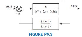
If the system of Figure P9.3 operates with a damping ratio of 0.456 for the dominant second-order poles, find the location of all closed-loop poles and zeros. R(s) K C(s) (s2 + 2s + 0.36) (s + 3) (s + 2) FIGURE P9.3
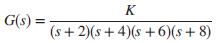
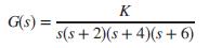
For the unity feedback system in Figure P9.1, withdo the following:a. Design rate feedback to yield a step response with no more than 15% overshoot and no more than 3 seconds settling time. Use Approach 1.b. Use MATLAB and simulate your compensated system. K G(s) = s(s + 2)(s + 4)(s + 6)
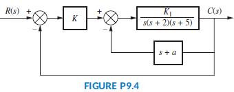
Given the system of Figure P9.4:a. Design the value of K1, as well as a in the feedback path of the minor loop, to yield a settling time of 4 seconds with 5% overshoot for the step response.b. Design the value of K to yield a major-loop response with 10% overshoot for a step input.c. Use MATLAB or
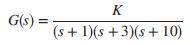
Design a PI controller to drive the step-response error to zero for the unity feedback system shown in Figure P9.1, whereThe system operates with a damping factor of 0.4. Design for each of the following two cases: (1) compensator zero at -0.1, and (2) compensator zero at -0.7. Compare the
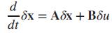
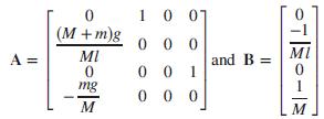
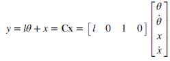
An inverted pendulum mounted on a motor-driven cart was introduced in Problem 30 in Chapter 3. Its state-space model was linearized around a stationary point, x0 = 0 (Prasad, 2012). At the stationary point, the pendulum point-mass, m, is in the upright position at t = 0, and the force applied to
Identify and realize the following controllers with operational amplifiers.a. s + 0.01/sb. s + 2
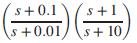
Identify and realize the following compensators with passive networks.a. s + 0.1/s + 0.01b. s + 2/s + 5c. (s+0.1 s+1 s+0.01 s+ 10
Repeat Problem 35 using operational amplifiers.Data From Problem 35:Identify and realize the following compensators with passive networks.a. s + 0.1/s + 0.01b. s + 2/s + 5c. (s+0.1 s+1 s+0.01 s+ 10
The room temperature of an 11 m2 room is to be controlled by varying the power of an indoor radiator. For this specific room, the open-loop transfer function from radiator power, Q̇ (s), to temperature, T(s), is (Thomas, 2005)The system is assumed to be in the closed-loop configuration shown in
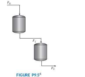
Figure P9.5 shows a two-tank system. The liquid inflow to the upper tank can be controlled using a valve and is represented by F0. The upper tank’s outflow equals the lower tank’s inflow and is represented by F1. The outflow of the lower tank is F2. The objective of the design is to control the
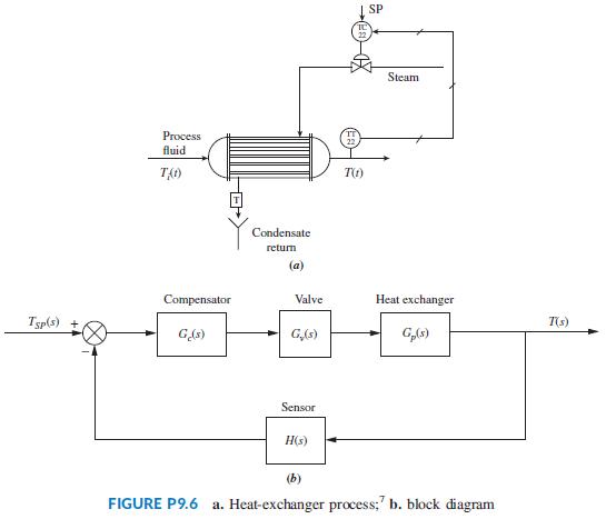
Figure P9.6(a) shows a heat-exchanger process whose purpose is to maintain the temperature of a liquid at a prescribed temperature. The temperature is measured using a sensor and a transmitter, TT 22, that sends the measurement to a corresponding controller,TC22, that compares the actual
Repeat Problem 39, Parts b and c, using a lead compensator.Data From Problem 39:Figure P9.6(a) shows a heat-exchanger process whose purpose is to maintain the temperature of a liquid at a prescribed temperature. The temperature is measured using a sensor and a transmitter, TT 22, that sends the
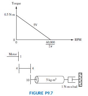
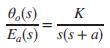
a. Find the transfer function of a motor whose torquespeed curve and load are given in Figure P9.7.b. Design a tachometer compensator to yield a damping ratio of 0.5 for a position control employing a power amplifier of gain 1 and a preamplifier of gain 5000.c. Compare the transient and
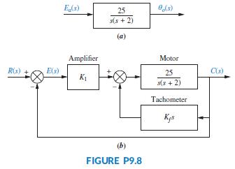
You are given the motor whose transfer function is shown in Figure P9.8(a).a. If this motor were the forward transfer function of a unity feedback system, calculate the percent overshoot and settling time that could be expected.b. You want to improve the closed-loop response. Since the motor
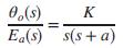
A position control is to be designed with a 20%overshoot and a settling time of 2 seconds. You have on hand an amplifier and a power amplifier whose cascaded transfer function is K1/(s + 20) with which to drive the motor. Two 10-turn pots are available to convert shaft position into voltage. A
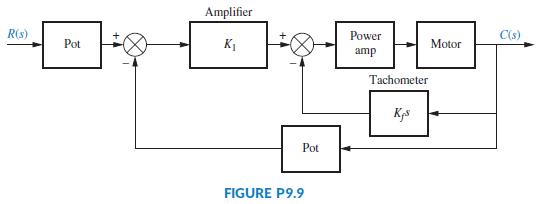
A position control is to be designed with a10%overshoot, a settling time of 1 second, and Kv = 1000. You have on hand an amplifier and a power amplifier whose cascaded transfer function is K1/(s + 40) with which to drive the motor. Two 10-turn pots are available to convert shaft position into
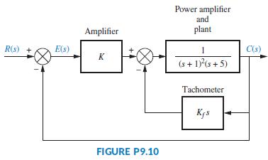
Given the system shown in Figure P9.10, find the values of K and Kf so that the closed-loop dominant poles will have a damping ratio of 0.5 and the underdamped poles of the minor loop will have a damping ratio of 0.8. Power amplifier and Amplifier plant R(s) E(s) C(s) K Tachometer Kys FIGURE P9.10
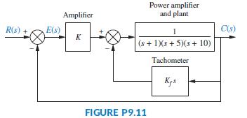
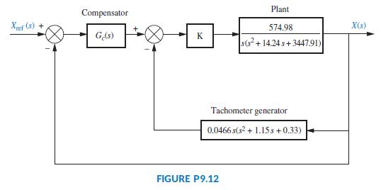
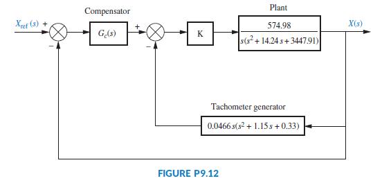
Given the system in Figure P9.11, find the values of K and Kf so that the closed-loop system will have a 4.32% overshoot and the minor loop will have a damping ratio of 0.8. Compare the expected performance of the system without tachometer compensation to the expected performance with tachometer
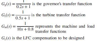
Steam-driven power generators rotate at a constant speed via a governor that maintains constant steam pressure in the turbine. In addition, automatic generation control (AGC) or load frequency control (LFC) is added to ensure reliability and consistency despite load variations or other disturbances
Repeat Problem47 using a lag-lead compensator instead of a PID controller. Design for a steady-state error of 1% for a step input command.Data From Problem 47:Steam-driven power generators rotate at a constant speed via a governor that maintains constant steam pressure in the turbine. In addition,
Digital versatile disc (DVD) players incorporate several control systems for their operations. The control tasks include (1) keeping the laser beam focused on the disc surface, (2) fast track selection, (3) disc rotation speed control, and (4) following a track accurately. In order to follow a
A coordinate measuring machine (CMM) measures coordinates on three-dimensional objects. The accuracy of CMMs is affected by temperature changes as well as by mechanical resonances due to joint elasticity. These resonances are more pronounced when the machine has to go over abrupt changes of
An X-4 quadrotor flyer is designed as a small-sized unmanned autonomous vehicle (UAV) that flies mainly indoor sand can help in search and recognizance missions. To minimize mechanical problems and for simplicity, this aircraft uses fixed pitch rotors with specially designed blades. Therefore, for
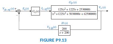
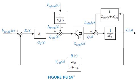
Problem 8.54 described an ac/dc conversion and power distribution system for which droop control is implemented through the use of a proportional controller to stabilize the dc-bus voltage. For simplification, a system with only one source converter and one load converter was considered. The
Testing of hypersonic flight is performed in wind tunnels where maintaining a constant air pressure is important. Air pressure control is accomplished in several stages. For a specific setup, a simplified transfer function has been found to be (Varghese, 2009)where M(s) is the stem movement of a
A metering pump is a pump capable of delivering a precise flow rate of fluid. Most metering pumps consist of an electric motor that varies the strike length of a shaft, allowing more or less fluid to pass through its body. The control of such a valve has been considered and the open loop transfer
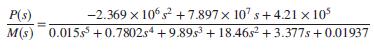
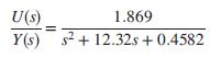
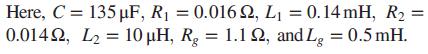
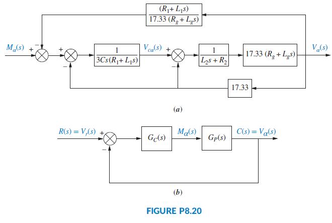
A linear model of the α-subsystem of a grid-connected converter (Mahmood, 2012) with a Y-Y transformer was presented as the plant in Problem 69 in Chapter 8. You were asked to find the transfer function of that plant, GP(s) = Vα(s)/Mα(s).a. Use the results of your solution to Problem 69, Chapter
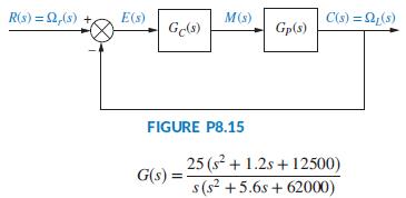
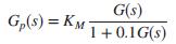
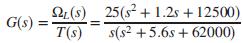
Design a PID controller for the drive system of Problem 56, Chapter 8, and shown in Figure P8.15 (Thomsen, 2011). Obtain an output response, ωL(t), with an overshoot 15%, a settling time of preferably 0.2 second, but not more than 5 seconds, a zero steady-state position error, and a velocity error
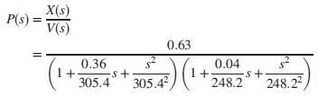
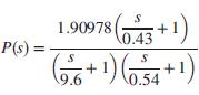
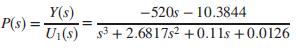
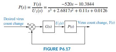
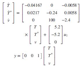
It was shown in Chapter 6, Problem 68, that when the virus levels in an HIV/ AIDS patient are controlled using RTIs the linearized plant model isAssume that the system is embedded in a configuration, such as the one shown in Figure P9.1, where G(s) = Gc(s) P(s). Here, Gc(s) is a cascade
Find analytical expressions for the magnitude and phase response for each G(s) below.a.b.c. 1 G(s) = s(s +2)(s+ 4)
Define frequency response as applied to a physical system.
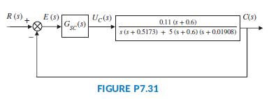
In the previous chapter, we used the root locus to design a proportional controller for the speed control of an HEV. We rearranged the block diagram to be a unity feedback system, as shown in the block diagram of Figure P7.31 (Preitl, 2007). The plant and compensator resulted inand we found that K
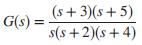
The parabolic trough collector (Camacho, 2012) is a Type 0 system as can be seen from its transfer function,We want the system operating in the critically damped mode, but with reduced steady-state error. Using the root locus and a Padé approximation,do the following:a. Substitute the Padé
Name four advantages of frequency response techniques over the root locus.
Name two ways to plot the frequency response.
Briefly describe how to obtain the frequency response analytically.
Define Bode plots.
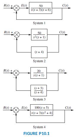
Sketch the Nyquist diagram for each of the systems in Figure P10.1. R(s) + E(s) 50 C(s) s(s + 3)(s + 6) System I R(s) + 50 C(s) s2(5 + 1) (s+ 4) System 2 R(s) + 20 C(s) s(s + 1) (s +3) (s+ 4) System 3 R(s) E(s) 100(s + 5) C(s) s(s + 3)(s2 + 4) System 4 FIGURE P10.1
Each pole of a system contributes how much of a slope to the Bode magnitude plot?
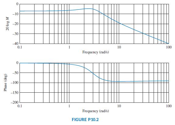
Draw the polar plot from the separate magnitude and phase curves shown in Figure P10.2. -10 -20 -30 -40 0.1 1 10 100 Frequency (rad/s) -50 -100 -150 -200 0.1 10 100 Frequency (rad/s) FIGURE P10.2 (Sap) əseyd 20 log M
A system with only four poles and no zeros would exhibit what value of slope at high frequencies in a Bode magnitude plot?
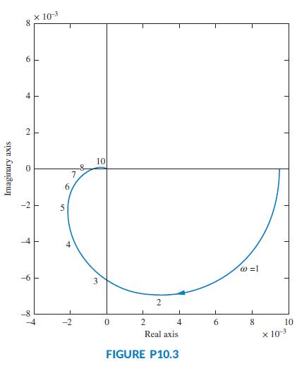
Draw the separate magnitude and phase curves from the polar plot shown in Figure P10.3. x 103 10 -& 7. 6. -6 2 4 8 10 Real axis x 103 FIGURE P10.3 2. 4. 6. 2. Imaginary axis
A system with four poles and two zeros would exhibit what value of slope at high frequencies in a Bode magnitude plot?
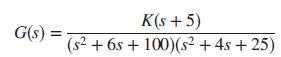
Write a program in MATLAB that will do the following:a. Plot the Nyquist diagram of a systemb. Display the real-axis crossing value and frequencyApply your program to a unity feedback system with K(s + 5) (s2 + 6s + 100)(s² +4s + 25) G(s) :
Describe the asymptotic phase response of a system with a single pole at 2.
What is the major difference between Bode magnitude plots for first-order systems and for second-order systems?
What does the Nyquist criterion tell us?
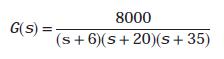
Use MATLAB’s LTI Viewer to find the gain margin, phase margin, zero dB frequency, and 180° frequency for a unity feedback system withUse the following methods:a. The Nyquist diagramb. Bode plots 8000 G(S) = (s + 6)(s+ 20)(s+ 35)
What is a Nyquist diagram?
Derive Eq. (10.54), the closed-loop bandwidth in terms of ζ and ωn of a two-pole system.
Why is the Nyquist criterion called a frequency response method?
For each closed-loop system with the following performance characteristics, find the closed-loop bandwidth:a. ζ = 0:2; Ts = 3 secondsb. ζ = 0:2; Tp = 3 secondsc. Ts = 4 seconds; Tp = 2 secondsd. ζ = 0:3; Tr = 4 seconds:
Write a program in MATLAB that will do the following:a. Allow a value of gain, K, to be entered from the keyboardb. Display the Bode plots of a system for the entered value of Kc. Calculate and display the gain and phase margin for the entered value of K Test your program on a unity feedback
Briefly state the Nyquist criterion.
For a system with three poles at 4, what is the maximum difference between the asymptotic approximation and the actual magnitude response?
When sketching a Nyquist diagram, what must be done with open-loop poles on the imaginary axis?
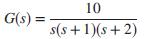
Consider the unity feedback system of Figure 10.10. For each G(s) that follows, use the M and N circles to make a plot of the closed-loop frequency response:a.b.c. 10 G(s) = s(s +1)(s+ 2)
What simplification to the Nyquist criterion can we usually make for systems that are open-loop stable?
What simplification to the Nyquist criterion can we usually make for systems that are open-loop unstable?
Using the results of Problem 16, estimate the percent overshoot that can be expected in the step response for each system shown.
Define gain margin.
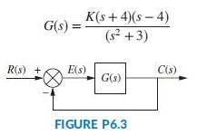
Find the range of K for stability for the unity feedback system of Figure P6.3 with K(s + 4)(s – 4) (s² +3) G(s) R(s) + E(s) C(s) G(s) FIGURE P6.3
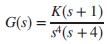
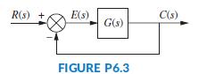
For the unity feedback system of Figure P6.3 withfind the range of K for stability. K(s + 1) G(s) = %3D
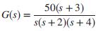
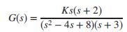
Given the unity feedback system of Figure P6.3 witha. Find the range of K for stability.b. Find the frequency of oscillation when the system is marginally stable. Ks(s + 2) (s2 – 4s + 8)(s + 3) G(s) =

Showing 300 - 400 of 942

1
2
3
4
5
6
7
8
9
10

Step by Step Answers

Services

Sitemap
Fun
Definitions
Become Tutor
Used Textbooks
Study Help Categories
Recent Questions
Expert Questions
Campus Wear
Sell Your Books

Company Info

Security
Copyrights
Privacy Policy
Terms & Conditions
SolutionInn Fee
Scholarship
Online Quiz
Give Feedback, Get Rewards

Get In Touch

About Us
Contact Us
Career
Jobs
FAQ
Student Discount
Campus Ambassador

Secure Payment

Download Our App

© 2026 SolutionInn. All Rights Reserved