New Semester
Started
Get
50% OFF
Study Help!
--h --m --s
Claim Now
Question Answers
Textbooks
Find textbooks, questions and answers
Oops, something went wrong!
Change your search query and then try again
S
Books
FREE
Study Help
Expert Questions
Accounting
General Management
Mathematics
Finance
Organizational Behaviour
Law
Physics
Operating System
Management Leadership
Sociology
Programming
Marketing
Database
Computer Network
Economics
Textbooks Solutions
Accounting
Managerial Accounting
Management Leadership
Cost Accounting
Statistics
Business Law
Corporate Finance
Finance
Economics
Auditing
Tutors
Online Tutors
Find a Tutor
Hire a Tutor
Become a Tutor
AI Tutor
AI Study Planner
NEW
Sell Books
Search
Search
Sign In
Register
study help
business
regression analysis
Introduction To Linear Regression Analysis 6th Edition Douglas C. Montgomery, Elizabeth A. Peck, G. Geoffrey Vining - Solutions
Suppose that the full model is \(y_{i}=\beta_{0}+\beta_{1} x_{i 1}+\beta_{2} x_{i 2}+\varepsilon_{i}, i=1,2, \ldots, n\), where \(x_{i 1}\) and \(x_{i 2}\) have been coded so that \(S_{11}=S_{22}=1\). We will also consider fitting a subset model, say \(y_{i}=\beta_{0}+\beta_{1} x_{i
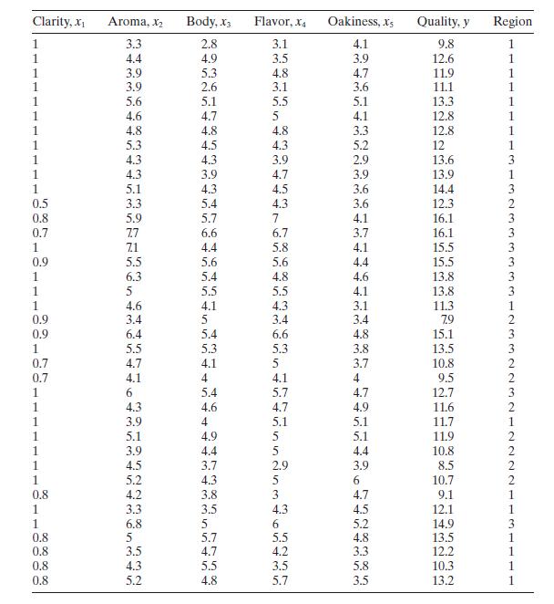
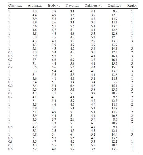
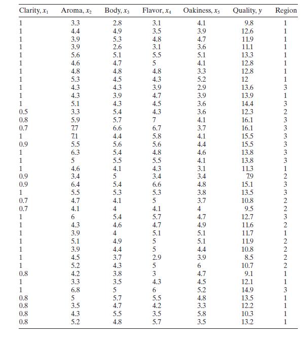
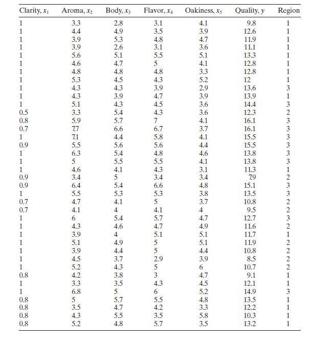
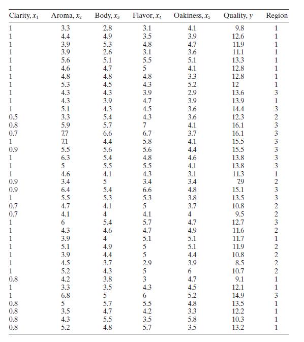
Table B. 11 presents data on the quality of Pinot Noir wine.a. Build an appropriate regression model for quality \(y\) using the all-possibleregressions approach. Use \(C_{p}\) as the model selection criterion, and incorporate the region information by using indicator variables.b. For the best two
Use the wine quality data in Table B. 11 to construct a regression model for quality using the stepwise regression approach. Compare this model to the one you found in Problem 10.4, part a.Data From Problem 10.4Consider the solar thermal energy test data in Table B.2. Clarity, x Aroma, X Body, X3
Rework Problem 10.14, part a, but exclude the region information.a. Comment on the difference in the models you have found. Is there indication that the region information substantially improves the model?b. Calculate confidence intervals as mean quality for all points in the data set using the
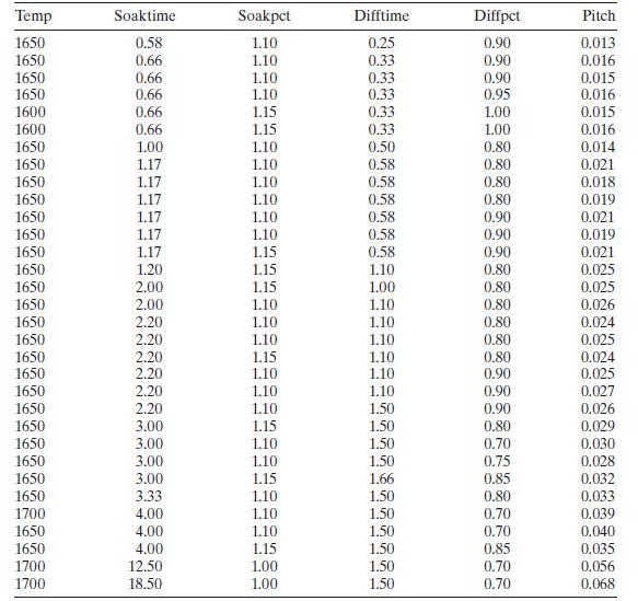
Table B. 12 presents data on a heat treating process used to carburize gears. The thickness of the carburized layer is a critical factor in overall reliability of this component. The response variable \(y=\) PITCH is the result of a carbon analysis on the gear pitch for a cross-sectioned part. Use
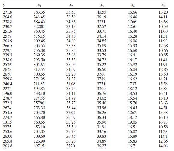
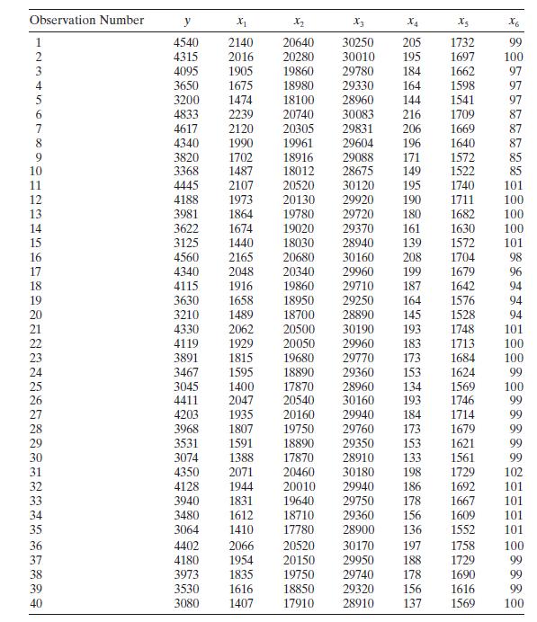
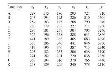
Table B. 13 presents data on the thrust of a jet turbine engine and six candidate regressors. Use all possible regressions and the \(C_{p}\) criterion to find an appropriate regression model for these data. Investigate model adequacy using residual plots. Observation Number y X x2 X3 X4 X5 1 4540
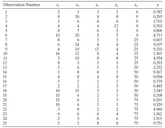
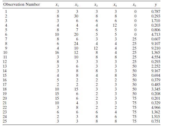
Table B. 14 presents data on the transient points of an electronic inverter. Use all possible regressions and the \(C_{p}\) criterion to find an appropriate regression model for these data. Investigate model adequacy using residual plots. Observation Number 1234567ERDURENDE 10 8 10 16 11 10 12 10
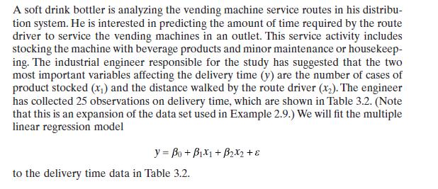
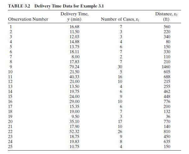
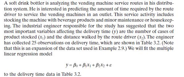
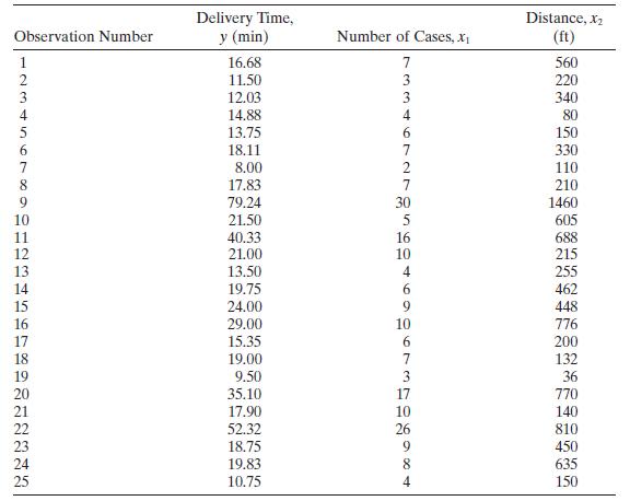
Consider the soft drink delivery time data in Example 3.1.Example 3.1a. Find the simple correlation between cases \(\left(x_{1}\right)\) an distance \(\left(x_{2}\right)\).b. Find the variance inflation factors.c. Find the condition number of \(\mathbf{X}^{\prime} \mathbf{X}\). Is there evidence of
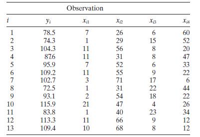
Consider the Hald cement data in Table B.21.a. From the matrix of correlations between the regressors, would you suspect that multicollinearity is present?b. Calculate the variance inflation factors.c. Find the eigenvalues of \(\mathbf{X}^{\prime} \mathbf{X}\).d. Find the condition number of
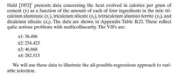
Using the Hald cement data (Example 10.1), find the eigenvector associated with the smallest eigenvalue of \(\mathbf{X}^{\prime} \mathbf{X}\). Interpret the elements of this vector. What can you say about the source of multicollinearity in these data?Data From Example 10.1 Hald [1952] presents data
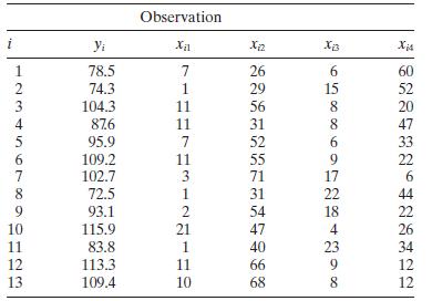
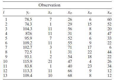
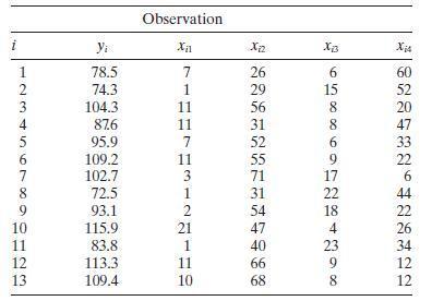
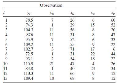
Find the condition indices and the variance decomposition proportions for the Hald cement data (Table B.21), assuming centered regressors. What can you say about multicollinearity in these data? Observation i Yi x12 Xiz 12345678 78.5 7 26 6 60 74.3 1 29 15 52 104.3 11 56 8 20 876 11 31 8 47 95.9
Repeat Problem 9.4 without centering the regressors and compare the results. Which approach do you think is better?Data From Problem 9.4Find the condition indices and the variance decomposition proportions for the Hald cement data (Table B.21), assuming centered regressors. What can you say about
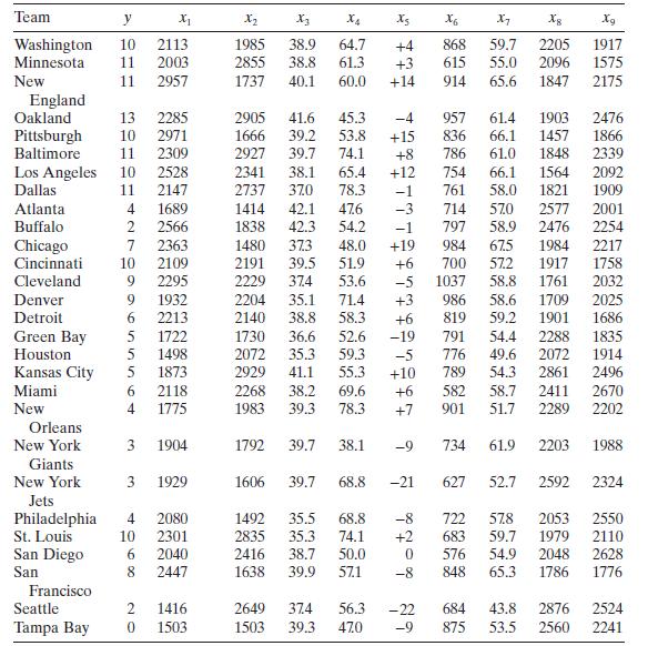
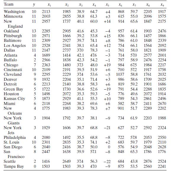
Use the regressors \(x_{2}\) (passing yardage), \(x_{7}\) (percentage of rushing plays), and \(x_{8}\) (opponents' yards rushing) for the National Football League data in Table B.1.a. Does the correlation matrix give any indication of multicollinearity?b. Calculate the variance inflation factors
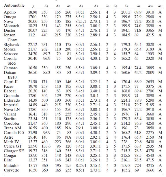
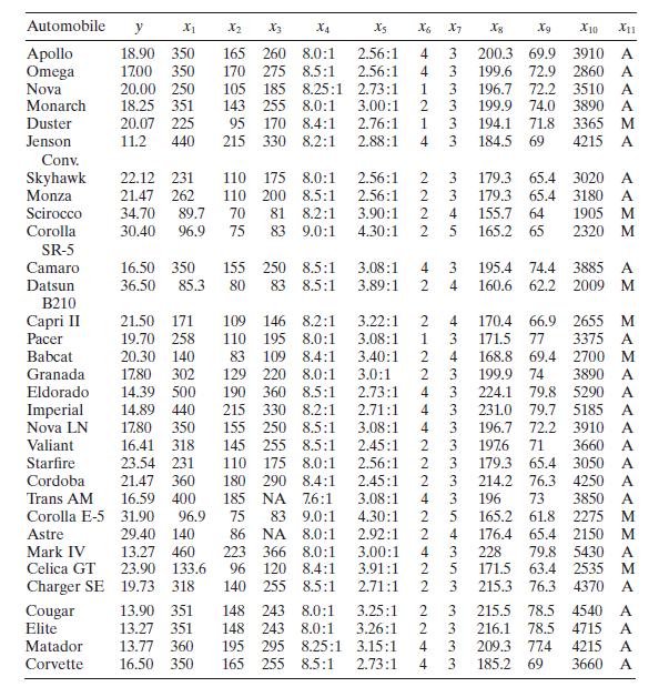
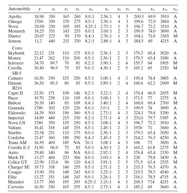
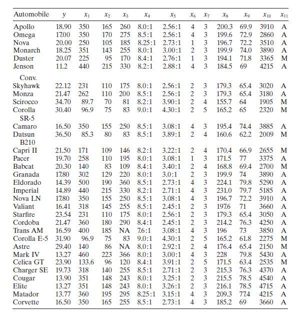
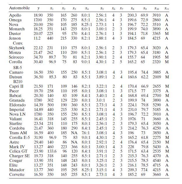
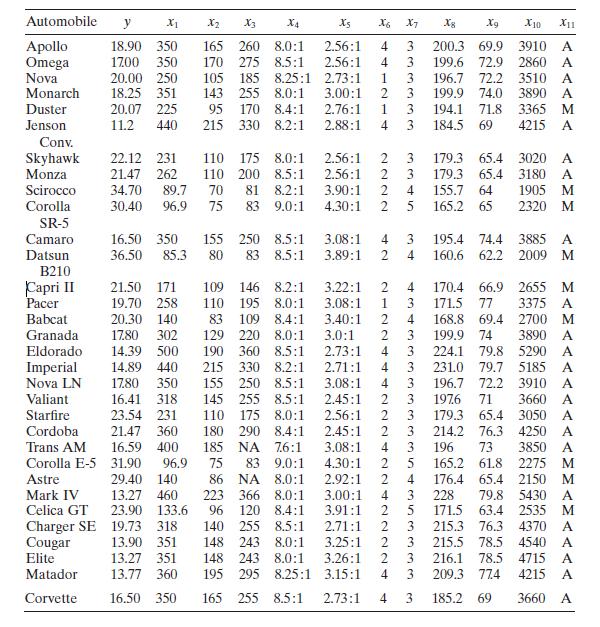
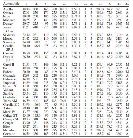
Consider the gasoline mileage data in Table B.3.a. Does the correlation matrix give any indication of multicollinearity?b. Calculate the variance inflation factors and the condition number of \(\mathbf{X}^{\prime} \mathbf{X}\). Is there any evidence of multicollinearity? Automobile y X1 X2 X3 X4 X5
Using the gasoline mileage data in Table B. 3 find the eigenvectors associated with the smallest eigenvalues of \(\mathbf{X}^{\prime} \mathbf{X}\). Interpret the elements of these vectors. What can you say about the source of multicollinearity in these data? Automobile y X2 X3 X4 Xs X6 X7 8 Xg X10
Use the gasoline mileage data in Table B. 3 and compute the condition indices and variance-decomposition proportions, with the regressors centered. What statements can you make about multicollinearity in these data? Automobile y X2 X3 X4 Xs X6 X7 8 Xg X10 X11 Apollo 18.90 350 165 260 8.0:1 2.56:1
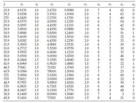
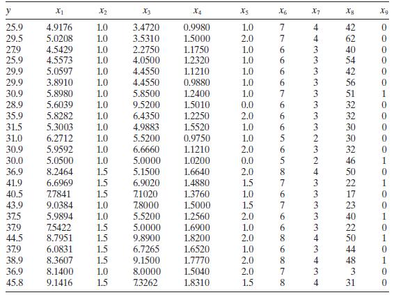
Analyze the housing price data in Table B. 4 for multicollinearity. Use the variance inflation factors and the condition number of \(\mathbf{X}^{\prime} \mathbf{X}\). y X1 X2 X3 X4 X5 X6 X7 Xg 25.9 4.9176 1.0 3.4720 0.9980 1.0 29.5 5.0208 1.0 3.5310 1.5000 2.0 27.9 4.5429 1.0 2.2750 1.1750 1.0
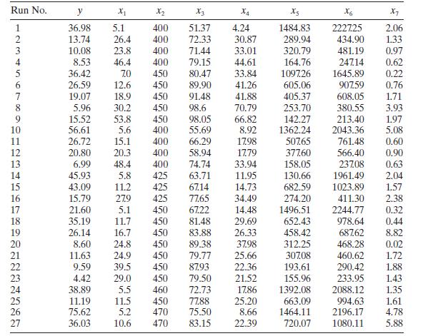
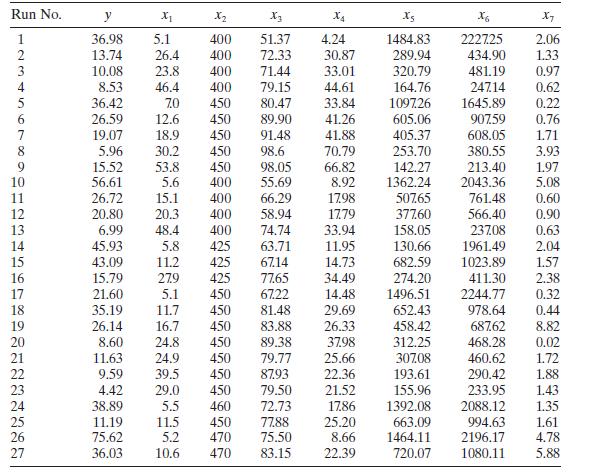
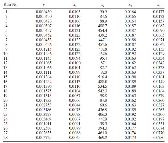
Analyze the chemical process data in Table B. 5 for evidence of multicollinearity. Use the variance inflation factors and the condition number of \(\mathbf{X}^{\prime} \mathbf{X}\). Run No. y X x2 X3 X4 Xs x6 X7 10 1234567890 36.98 5.1 400 51.37 4.24 1484.83 2227.25 2.06 13.74 26.4 400 72.33 30.87
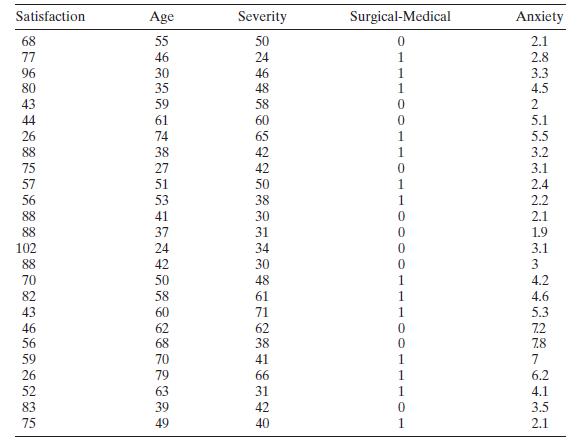
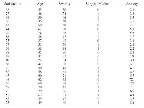
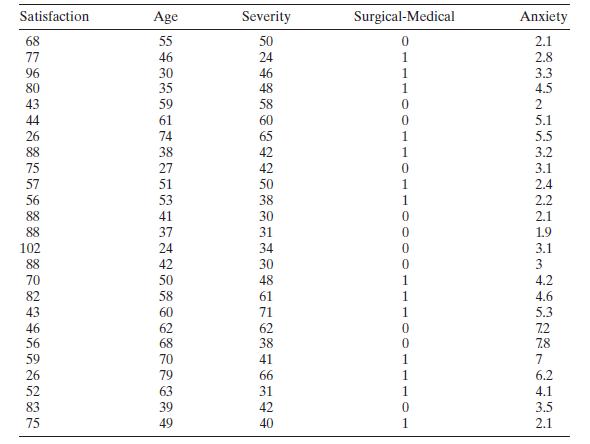
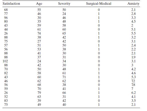
Analyze the patient satisfaction data in Table B. 17 for multicollinearity. Satisfaction Age Severity Surgical-Medical Anxiety 68 55 50 0 2.1 77 46 24 1 2.8 96 30 46 1 3.3 80 35 48 1 4.5 43 59 58 0 2 44 61 0 5.1 26 74 88 38 75 27 57 51 56 53 41 88 37 102 24 88 42 70 82 43 46 56 59 26 52 83 75 49
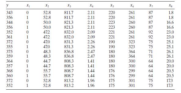
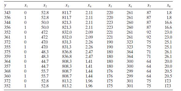
Analyze the fuel consumption data in Table B. 18 for multicollinearity. y X2 X3 X4 xs X6 X7 Xg 343 0 52.8 811.7 2.11 220 261 87 1.8 356 1 52.8 811.7 2.11 220 261 87 1.8 344 0 50.0 821.3 2.11 223 260 87 16.6 356 1 50.0 821.3 2.11 223 260 87 16.6 352 0 47.2 832.0 2.09 221 261 92 23.0 361 1 47.2
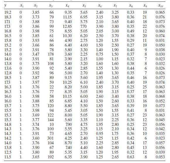
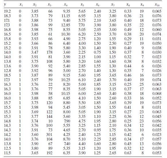
Analyze the wine quality of young red wines data in Table B. 19 for multicollinearity. y X2 X3 X4 x6 X7 Xg Xg x10 19.2 0 3.85 66 9.35 5.65 2.40 3.25 0.33 19 0.065 18.3 0 3.73 79 11.15 6.95 3.15 3.80 0.36 21 0.076 171 0 3.88 73 9.40 5.75 2.10 3.65 0.40 18. 0.073 173 0 3.86 99 12.85 7.70 3.90 3.80
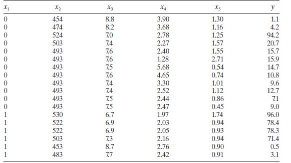
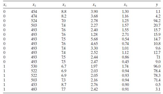
Analyze the methanol oxidation data in Table B. 20 for multicollinearity. x1 X2 X3 X4 xs 0 454 8.8 3.90 1.30 1.1 474 8.2 3.68 1.16 4.2 524 7.0 2.78 1.25 94.2 503 7.4 2.27 1.57 20.7 493 7.6 2.40 1.55 15.7 493 7.6 1.28 2.71 15.9 493 7.5 5.68 0.54 14.7 493 7.6 4.65 0.74 10.8 493 7.4 3.30 1.01 9.6 493
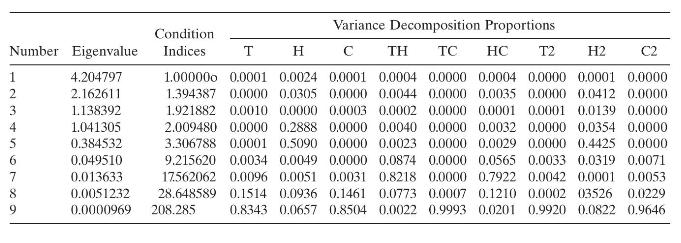
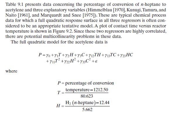
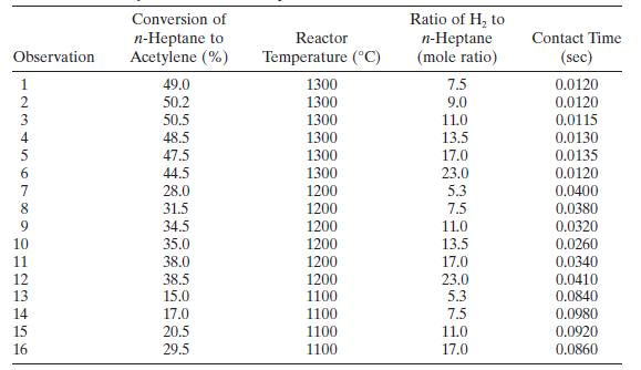
The table below shows the condition indices and variance decomposition proportions for the acetylene data using centered regressors. Use this information to diagnose multicollinearity in the data and draw appropriate conclusions. Condition 123456789 Number Eigenvalue Indices 4.204797 2.162611
Apply ridge regression to the Hald cement data in Table B.21.a. Use the ridge trace to select an appropriate value of \(k\). Is the final model a good one?b. How much inflation in the residual sum of squares has resulted from the use of ridge regression?c. Compare the ridge regression model with
Use ridge regression on the Hald cement data (Table B.21) using the value of \(k\) in Eq. (9.8). Compare this value of \(k\) value selected by the ridge trace in Problem 9.17. Does the final model differ greatly from the one in Problem 9.17?eq(9.8)Data From Problem 9.17Apply ridge regression to the
Estimate the parameters in a model for the gasoline mileage data in Table B. 3 using ridge regression.a. Use the ridge trace to select an appropriate value of \(k\). Is the resulting model adequate?b. How much inflation in the residual sum of squares has resulted from the use of ridge regression?c.
Estimate the parameters in a model for the gasoline mileage data in Table B. 3 using ridge regression with the value of \(k\) determined by Eq. (9.8). Does this model differ dramatically from the one developed in Problem 9.19?Eq (9.8)Data From Problem 9.19Estimate the parameters in a model for the
Estimate model parameters for the Hald cement data (Table B.21) using principal-component regression.a. What is the loss in \(R^{2}\) for this model compared to least squares?b. How much shrinkage in the coefficient vector has resulted?c. Compare the principal-component model with the ordinary
Estimate the model parameters for the gasoline mileage data using principalcomponent regression.a. How much has the residual sum of squares increased compared to least squares?b. How much shrinkage in the coefficient vector has resulted?c. Compare the principal-component and ordinary ridge models
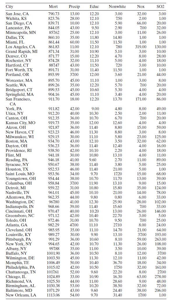
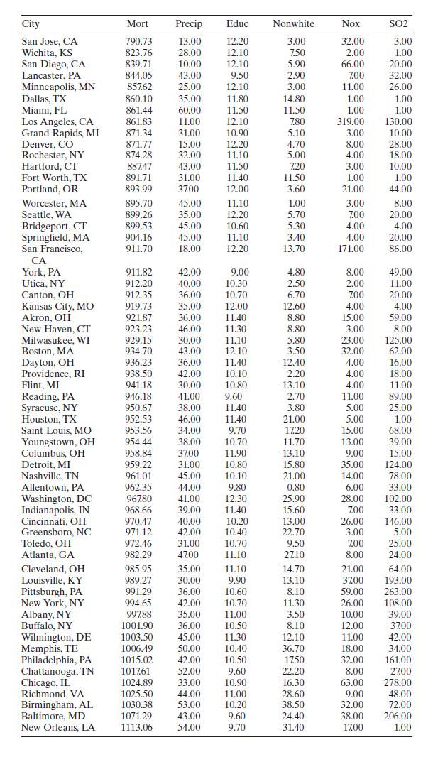
Consider the air pollution and mortality data given in Table B.15.a. Is there a problem with collinearity? Discuss how you arrived at this decision.b. Perform a ridge trace on these data.c. Select a \(k\) based upon the ridge trace from part \(b\). Which estimates of the coefficients do you prefer
Consider the air pollution and mortality data given in Table B.15.a. Is there a problem with collinearity? Discuss how you arrived at this decision.b. Perform a ridge trace on these data.c. Select a \(k\) based upon the ridge trace from part \(b\). Which estimates of the coefficients do you prefer
The pure shrinkage estimator is defined as \(\hat{\beta}_{s}=c \hat{\beta}\), were \(0 \leq c \leq 1\) is a constant chosen by the analyst. Describe the kind of shrinkage that this estimator introduces, and compare it with the shrinkage that results from ridge regression. Intuitively, which
Show that the pure shrinkage estimator (Problem 9.25) is the solution toData From Problem 9.25The pure shrinkage estimator is defined as \(\hat{\beta}_{s}=c \hat{\beta}\), were \(0 \leq c \leq 1\) is a constant chosen by the analyst. Describe the kind of shrinkage that this estimator introduces,
The mean square error criterion for ridge regression is\[E\left(L_{1}^{2}\right)=\sum_{j=1}^{p} \frac{\lambda_{j}}{\left(\lambda_{j}+k\right)^{2}}+\sum_{j=1}^{p} \frac{\alpha_{j}^{2} k^{2}}{\left(\lambda_{j}+k\right)^{2}}\]Try to find the value of \(k\) that minimizes \(E\left(L_{1}^{2}\right)\).
Consider the mean square error criterion for generalized ridge regression. Show that the mean square error is minimized by choosing \(k_{j}=\sigma^{2} / \alpha_{j}^{2}, j=1\), \(2, \ldots, p\).
Show that if \(\mathbf{X}^{\prime} \mathbf{X}\) is in correlation form, \(\boldsymbol{\Lambda}\) is the diagonal matrix of eigenvalues of \(\mathbf{X}^{\prime} \mathbf{X}\), and \(\mathbf{T}\) is the corresponding matrix of eigenvectors, then the variance inflation factors are the main diagonal
Formally show that\[D_{i}=\frac{r_{i}}{p} \frac{h_{i i}}{1-h_{i i}}\]
Table B. 14 contains data concerning the transient points of an electronic inverter. Fit a regression model to all 25 observations but only use \(x_{1}-x_{4}\) as the regressors. Investigate this model for influential observations and comment on your findings. Observation Number x x2 X3 Xs y
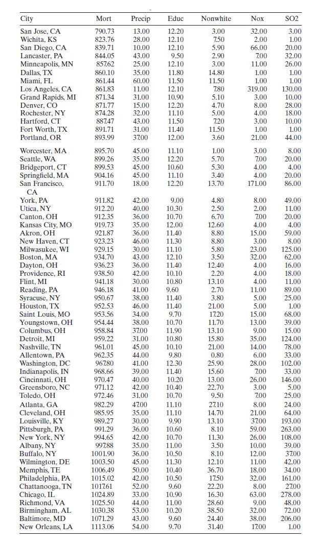
Perform a thorough influential analysis of the air pollution and mortality data given in Table B.15. Perform any appropriate transformations. Discuss your results. City Mort Precip Educ Nonwhite Nox SO2 San Jose, CA 790.73 13.00 12.20 3.00 32.00 3.00 Wichita, KS 823.76 28.00 12.10 7.50 2.00 1.00
Consider the patient satisfaction data in Table B.17. Fit a regression model to the satisfaction response using age and severity as the predictors. Perform an influence analysis of the date and comment on your findings. Satisfaction Age Severity Surgical-Medical Anxiety 0 1 56 59 1332 3999222-8787
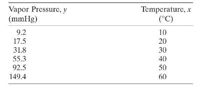
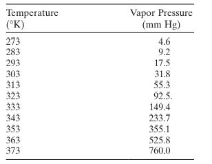
Chemical and mechanical engineers often need to know the vapor pressure of water at various temperatures (the "infamous" steam tables can be used for this). Below are data on the vapor pressure of water \((y)\) at various temperatures.a. Fit a first-order model to the data. Overlay the fitted model
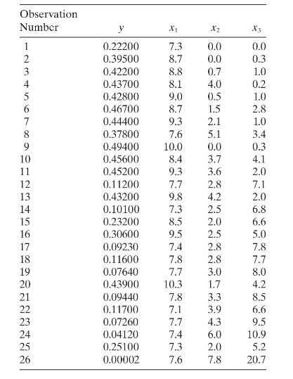
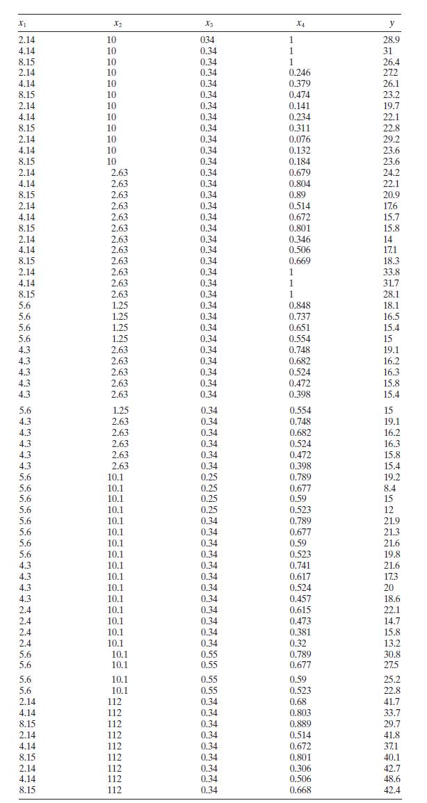
An article in the Journal of Pharmaceutical Sciences \((\mathbf{8 0}, 971-977,1991)\) presents data on the observed mole fraction solubility of a solute at a constant temperature, along with \(x_{1}=\) dispersion partial solubility, \(x_{2}=\) dipolar partial solubility, and \(x_{3}=\) hydrogen
Pet-Pro is a company that imports and markets pet food feeders to customers in Malaysia. The food feeder, which is called "Smart Feeder," allows pet owners to feed pre-determined quantities of food at pre-set times to their pets. The system has builtin webcam and Wi-Fi technology, allowing the pet
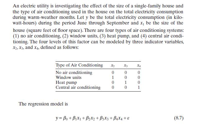
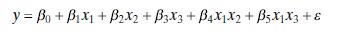
Consider the regression model (8.8) described in Example 8.3 Graph the response function for this model and indicate the role the model parameters play in determining the shape of this function.Example 8.3 An electric utility is investigating the effect of the size of a single-family house and the
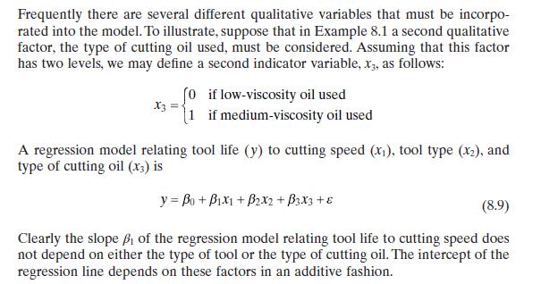
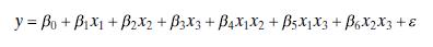
Consider the regression models described in Example 8.4.Example 8.4a. Graph the response function associated with Eq. (8.10).Equation (8.10)b. Graph the response function associated with Eq. (8.11).Equation (8.11) Frequently there are several different qualitative variables that must be incorpo-
Consider the delivery time data in Example 3.1. In Section 4.2.5 noted that these observations were collected in four cities, San Diego, Boston, Austin, and Minneapolis.Example 3.1 a. Develop a model that relates delivery time \(y\) to cases \(x_{1}\), distance \(x_{2}\), and the city in which the
Consider the automobile gasoline mileage data in Table B.3.a. Build a linear regression model relating gasoline mileage \(y\) to engine displacement \(x_{1}\) and the type of transmission \(x_{11}\). Does the type of transmission significantly affect the mileage performance?b. Modify the model
Consider the automobile gasoline mileage data in Table B.3.a. Build a linear regression model relating gasoline mileage $y$ to vehicle weight $x_{10}$ and the type of transmission $x_{11}$. Does the type of transmission significantly affect the mileage performance?b. Modify the model developed in
Consider the National Football League data in Table B.1. Build a linear regression model relating the number of games won to the yards gained rushing by opponents $x_{8}$, the percentage of rushing plays $x_{7}$, and a modification of the turnover differential $x_{5}$. Specifically let the turnover
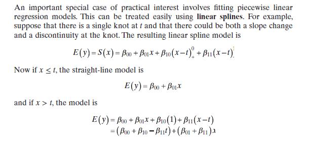
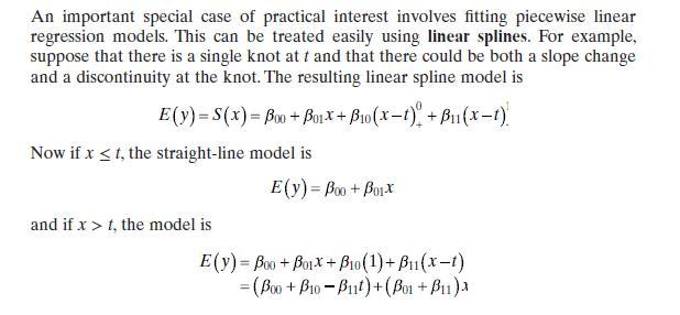
Piecewise Linear Regression. In Example 7.3 we showed how a linear regression model with a change in slope at some point $t\left(x_{\min }Example 7.3 An important special case of practical interest involves fitting piecewise linear regression models. This can be treated easily using linear
Continuation of Problem 8.7 . Show how indicator variables can be used to develop a piecewise linear regression model with a discontinuity at the join point $t$.Problem 8.7Piecewise Linear Regression. In Example 7.3 we showed how a linear regression model with a change in slope at some point
Suppose that a one-way analysis of variance involves four treatments but that a different number of observations (e.g., $n_{i}$ ) has been taken under each treatment. Assuming that $n_{1}=3, n_{2}=2, n_{3}=4$, and $n_{4}=3$, write down the $\mathbf{y}$ vector and $\mathbf{X}$ matrix for analyzing
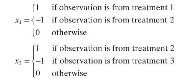
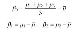
Alternate Coding Schemes for the Regression Approach to Analysis of Variance. Consider Eq. (8.18), which represents the regression model corresponding to an analysis of variance with three treatments and $n$ observations per treatment. Suppose that the indicator variables $x_{1}$ and $x_{2}$ are
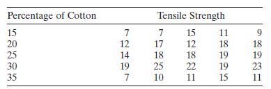
Montgomery [2020] presents an experiment concerning the tensile strength of synthetic fiber used to make cloth for men's shirts: The strength is thought to be affected by the percentage of cotton in the fiber. The data are shown below.a. Write down the $\mathbf{y}$ vector and $\mathbf{X}$ matrix
Two-Way Analysis of Variance. Suppose that two different sets of treatments are of interest. Let \(y_{i j k}\) be the \(k\) th observation level \(i\) of the first treatment type and level \(j\) of the second treatment type. The two-way analysis-ofvariance model is\[\begin{aligned}& y_{i j
Table B. 11 presents data on the quality of Pinot Noir wine.a. Build a regression model relating quality \(y\) to flavor \(x_{4}\) that incorporates the region information given in the last column. Does the region have an impact on wine quality?b. Perform a residual analysis for this model and
Using the wine quality data from Table B.11, fit a model relating wine quality $y$ to flavor $x_{4}$ using region as an allocated code, taking on the values shown in the table $(1,2,3)$. Discuss the interpretation of the parameters in this model. Compare the model to the one you built using
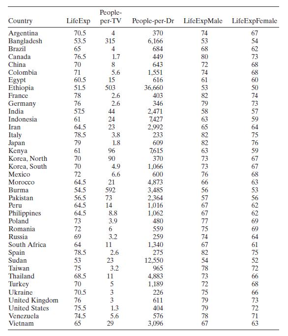
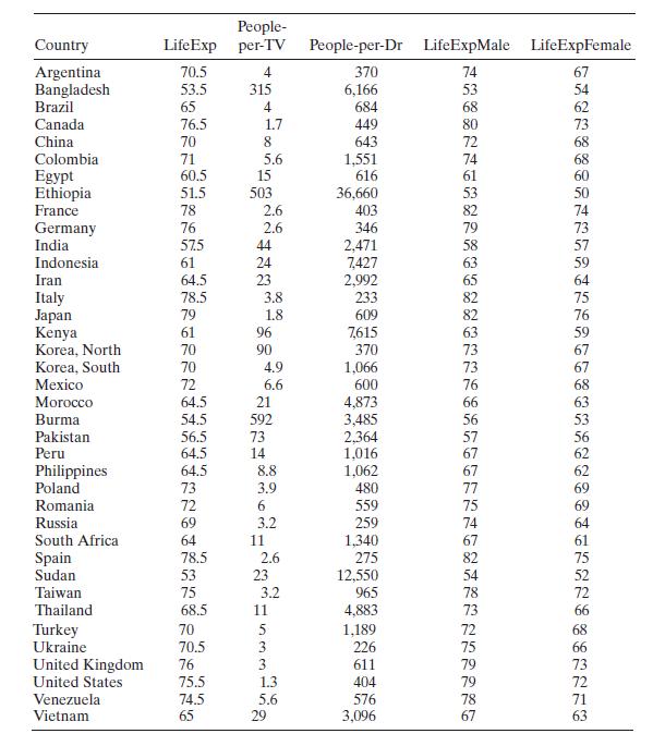
Consider the life expectancy data given in Table B.16. Create an indicator variable for gender. Perform a thorough analysis of the overall average life expectancy. Discuss the results of this analysis relative to your previous analyses of these data. People- Country Argentina Life Exp per-TV
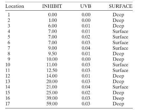
Smith et al. [1992] discuss a study of the ozone layer over the Antarctic. These scientists developed a measure of the degree to which oceanic phytoplankton production is inhibited by exposure to ultraviolet radiation (UVB). The response is INHIBIT. The regressors are UVB and SURFACE, which is
Table B. 17 contains hospital patient satisfaction data. Fit an appropriate regression model to the satisfaction response using age and severity as the regressors and account for the medical versus surgical classification of each patient with an indicator variable. Has adding the indicator variable
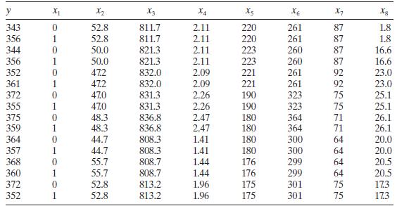
Consider the fuel consumption data in Table B.18. Regressor \(x_{1}\) is an indicator variable. Perform a thorough analysis of these data. What conclusions do you draw from this analysis? y X2 X3 X4 6 X7 Xg 343 0 52.8 811.7 2.11 220 261 87 1.8 356 1 52.8 811.7 2.11 220 261 87 1.8 344 0 50.0 821.3
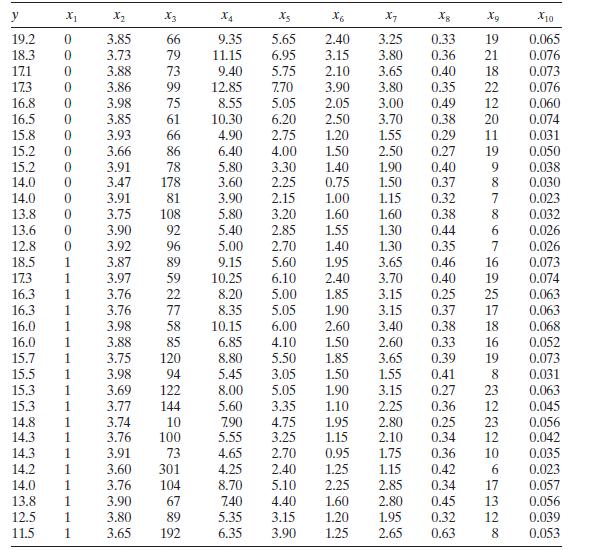
Consider the wine quality of young red wines data in Table B.19. Regressor $x_{1}$ is an indicator variable. Perform a thorough analysis of these data. What conclusions do you draw from this analysis? y X2 X3 X4 X5 X6 X7 Xg X10 19.2 0 3.85 66 9.35 5.65 2.40 3.25 0.33 19 0.065 18.3 0 3.73 79 11.15
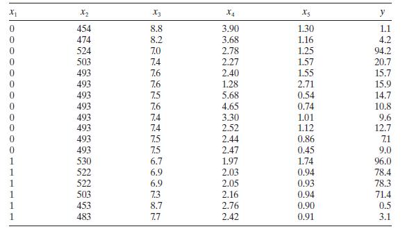
Consider the methanol oxidation data in Table B.20. Perform a thorough analysis of these data. What conclusions do you draw from this analysis? x x2 3 X4 Xs y 0 454 8.8 3.90 1.30 1.1 0 474 8.2 3.68 1.16 4.2 0 524 7.0 2.78 1.25 94.2 0 503 7.4 2.27 1.57 20.7 0 493 7.6 2.40 1.55 15.7 0 493 7.6 1.28
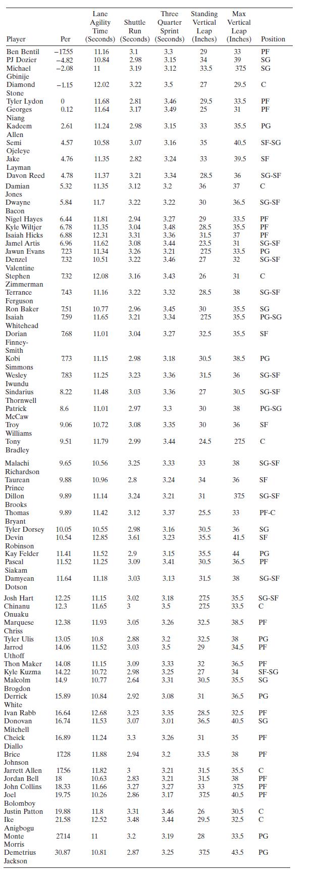
Table B.23 contains player efficiency ratings (PER) from the 2016-17 and 2017-18 NBA combine that evaluates 60 rookies hoping to be drafted by NBA teams. PER is a measure of a player's per-minute productivity that is a summation of positive contribution (such as points and assists) and minus
Use the NBA PER data introduced in Problem 8.21 and consider the model found in part $\mathrm{c}$ of that problem. There are some potential outliers in the data (the first observation is an obvious outlier). Remove the outliers and refit the model. Did removing the outliers improve the model?Data
Use the NBA PER data introduced in Problem 8.21 and consider the model found in Problem 8.22. After the outliers are removed it is not obvious that all of the terms in the model are important. Refine the model by removing any regressors that you think are unnecessary. Does this result in an
The following table gives the vapor pressure of water for various temperaturesa. Plot a scatter diagram. Does it seem likely that a straight-line model will be adequate? b. Fit the straight-line model. Compute the summary statistics and the residual plots. What are your conclusions regarding model
Consider the three modelsa. \(y=\beta_{0}+\beta_{1}(1 / x)+\varepsilon\)b. \(1 / y=\beta_{0}+\beta_{1} x+\varepsilon\)c. \(y=x /\left(\beta_{0}-\beta_{1} x\right)+\varepsilon\)All of these models can be linearized by reciprocal transformations. Sketch the behavior of \(y\) as a function of \(x\).
How are databases useful for managers?
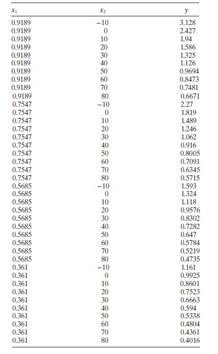
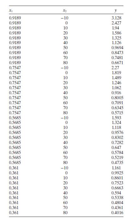
Consider the kinematic viscosity data in Table B.10.a. Perform a thorough residual analysis of these data.b. Identify the most appropriate transformation for these data. Fit this model and repeat the residual analysis. X1 X2 y 0.9189 -10 3.128 0.9189 0 2.427 0.9189 10 1.94 0.9189 20 1.586 0.9189 30
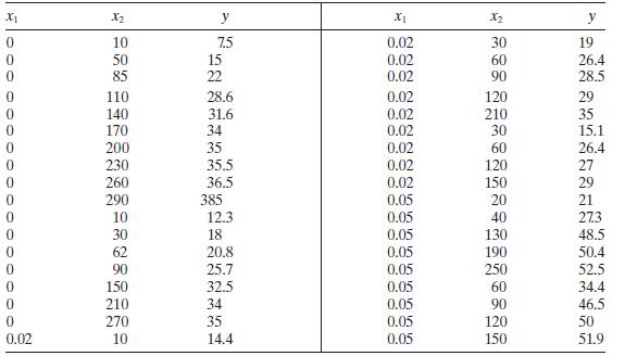
French and Schultz ("Water Use Efficiency of Wheat in a Mediterranean-type Environment, I The Relation between Yield, Water Use, and Climate," Australian Journal of Agricultural Research, 35, 743-64) studied the impact of water use on the yield of wheat in Australia. The data below are from 1970
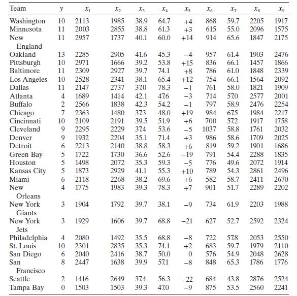
Consider the National Football League data in Table B.1.a. Fit a multiple linear regression model relating the number of games won to the team's passing yardage $\left(x_{2}\right)$, the percentage of rushing plays $\left(x_{7}\right)$, and the opponents' yards rushing $\left(x_{8}\right)$.b.
Using the results of Problem 3.1, show numerically that the square of the simple correlation coefficient between the observed values $y_{i}$ and the fitted values $\hat{y}_{i}$ equals $R^{2}$.Data From Problem 3.1Consider the National Football League data in Table B.1. Team y X_ X2 X4 X5 X6 5 X7 8
Refer to Problem 3.1.Data From Problem 3.1Consider the National Football League data in Table B.1.a. Find a $95 % \mathrm{CI}$ on $\beta_{7}$.b. Find a $95 %$ CI on the mean number of games won by a team when $x_{2}=2300, x_{7}=56.0$, and $x_{8}=2100$. Team y X_ X2 X4 X5 X6 5 X7 8 Xg Washington 10
Reconsider the National Football League data from Problem 3.1. Fit a model to these data using only $x_{7}$ and $x_{8}$ as the regressors.Data From Problem 3.1Consider the National Football League data in Table B.1.a. Test for significance of regression.b. Calculate $R^{2}$ and $R_{\text {Adj
Consider the gasoline mileage data in Table B.3.a. Fit a multiple linear regression model relatmg gasoline mileage $y$ (miles per gallon) to engine displacement $x_{1}$ and the number of carburetor barrels $x_{6}$.b. Construct the analysis-of-variance table and test for significance of
In Problem 2.4 you were asked to compute a $95 %$ CI on mean gasoline prediction interval on mileage when the engine displacement $x_{1}=275$ in. $^{3}$ Compare the lengths of these intervals to the lengths of the confidence and prediction intervals from Problem 3.5 above. Does this tell you
Consider the house price data in Table B.4.a. Fit a multiple regression model relating selling price to all nine regressors.b. Test for significance of regression. What conclusions can you draw?c. Use $t$ tests to assess the contribution of each regressor to the model. Discuss your findings.d. What
The data in Table B. 5 present the performance of a chemical process as a function of several controllable process variables.a. Fit a multiple regression model relating $\mathrm{CO}_{2}$ product $(y)$ to total solvent $\left(x_{6}\right)$ and hydrogen consumption $\left(x_{7}\right)$.b. Test for
The concentration of $\mathrm{NbOCl}_{3}$ in a tube-flow reactor as a function of several controllable variables is shown in Table B.6.a. Fit a multiple regression model relating concentration of $\mathrm{NbOCl}_{3}(y)$ to concentration of $\mathrm{COCl}_{2},\left(x_{1}\right)$ and mole fraction
The quality of Pinot Noir wine is thought to be related to the properties of clarity, aroma, body, flavor, and oakiness. Data for 38 wines are given in Table B. 11 .a. Fit a multiple linear regression model relating wine quality to these regressors.b. Test for significance of regression. What
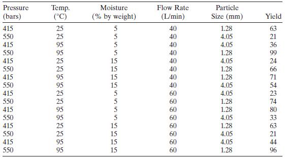
An engineer performed an experiment to determine the effect of $\mathrm{CO}_{2}$ pressure, $\mathrm{CO}_{2}$ temperature, peanut moisture, $\mathrm{CO}_{2}$ flow rate, and peanut particle size on the total yield of oil per batch of peanuts. Table B. 7 summarizes the experimental results.a. Fit a
A chemical engineer studied the effect of the amount of surfactant and time on clathrate formation. Clathrates are used as cool storage media. Table B. 8 summarizes the experimental results.a. Fit a multiple linear regression model relating clathrate formation to these regressors.b. Test for
An engineer studied the effect of four variables on a dimensionless factor used to describe pressure drops in a screen-plate bubble column. Table B. 9 summarizes the experimental results.a. Fit a multiple linear regression model relating this dimensionless number to these regressors.b. Test for
The kinematic viscosity of a certain solvent system depends on the ratio of the two solvents and the temperature. Table B. 10 summarizes a set of experimental results.a. Fit a multiple linear regression model relating the viscosity to the two regressors.b. Test for significance of regression. What
McDonald and Ayers [1978] present data from an early study that examined the possible link between air pollution and mortality. Table B. 15 summarizes the data. The response MORT is the total age-adjusted mortality from allcauses, in deaths per 100,000 population. The regressor PRECIP is the mean
Rossman [1994] presents an interesting study of average life expectancy of 40 countries. Table B. 16 gives the data. The study has three responses: LifeExp is the overall average life expectancy. LifeExpMale is the average life expectancy for males, and LifeExpFemale is the average life expectancy
Consider the patient satisfaction data in Table B.17. For the purposes of this exercise, ignore the regressor "Medical-Surgical." Perform a thorough analysis of these data. Please discuss any differences from the analyses outlined in Sections 2.7 and 3.6. Satisfaction Age Severity Surgical-Medical
Consider the fuel consumption data in Table B.18. For the purposes of this exercise, ignore regressor $x_{1}$. Perform a thorough analysis of these data. What conclusions do you draw from this analysis? y X X2 X3 X4 Xs X6 X7 Xg 343 0 52.8 811.7 2.11 220 261 87 1.8 356 1 52.8 811.7 2.11 220 261 87
Consider the wine quality of young red wines data in Table B.19. For the purposes of this exercise, ignore regressor $x_{1}$. Perform a thorough analysis of these data. What conclusions do you draw from this analysis? y X2 X3 x4 X5 X6 X7 Xg X10 19.2 0 3.85 66 9.35 5.65 2.40 3.25 0.33 19 0.065 18.3
Consider the methanol oxidation data in Table B.20. Perform a thorough analysis of these data. What conclusions do you draw from this analysis? x x2 X3 X4 y 0 454 8.8 3.90 1.30 1.1 0 474 8.2 3.68 1.16 4.2 0 524 7.0 2.78 1.25 94.2 0 503 7.4 2.27 1.57 20.7 0 493 7.6 2.40 1.55 15.7 0 493 7.6 1.28 2.71
Show that an alternate computing formula for the regression sum of squares in a linear regression model is \[S S_{\mathrm{R}}=\sum_{i=1}^{n} \hat{y}_{i}^{2}-n \bar{y}^{2}\]
Consider the multiple linear regression model \[ y=\beta_{0}+\beta_{1} x_{1}+\beta_{2} x_{2}+\beta_{3} x_{3}+\beta_{4} x_{4}+\varepsilon \] Using the procedure for testing a general linear hypothesis, show how to testa. $H_{0}: \beta_{1}=\beta_{2}=\beta_{3}=\beta_{4}=\beta$b. $H_{0}:
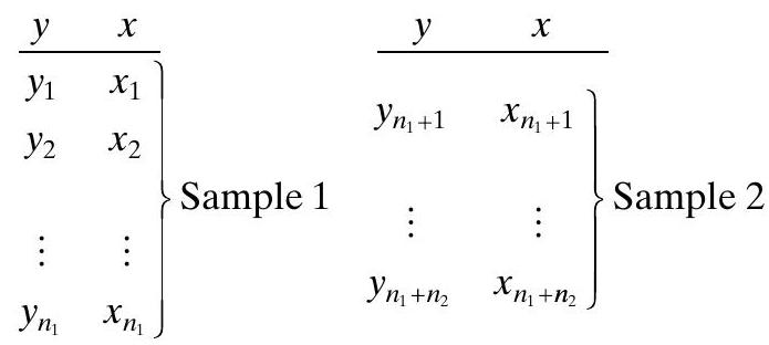
Suppose that we have two independent samples, sayTwo models can be fit to these samples,\[\begin{gathered}y_{i}=\beta_{0}+\beta_{1} x_{i}+\varepsilon_{i}, \quad i=1,2, \ldots, n_{2} \\y_{i}=\gamma_{0}+\gamma_{1} x_{i}+\varepsilon_{i}, \quad i=n_{1}+1, n_{1}+2, \ldots, n_{1}+n_{2}\end{gathered}\]a.
Show that $\operatorname{Var}(\hat{\mathbf{y}})=\sigma^{2} \mathbf{H}$.
Prove that the matrices $\mathbf{H}$ and $\mathbf{I}-\mathbf{H}$ are idempotent, that is, $\mathbf{H H}=\mathbf{H}$ and $(\mathbf{I}-\mathbf{H})(\mathbf{I}-\mathbf{H})=\mathbf{I}-\mathbf{H}$.
For the simple linear regression model, show that the elements of the hat matrix are\[h_{i j}=\frac{1}{n}+\frac{\left(x_{i}-\bar{x}\right)\left(x_{j}-\bar{x}\right)}{S_{x x}} \text { and } h_{i i}=\frac{1}{n}+\frac{\left(x_{i}-\bar{x}\right)^{2}}{S_{x x}}\]Discuss the behavior of these quantities
Consider the multiple linear regression model $\mathbf{y}=\mathbf{X} \boldsymbol{\beta}+\boldsymbol{\varepsilon}$. Show that the least-squares estimator can be written as\[\hat{\beta}=\beta+\mathbf{R} \varepsilon \quad \text { where } \quad \mathbf{R}=\left(\mathbf{X}^{\prime}
Show that the residuals from a linear regression model can be expressed as $\mathbf{e}=(\mathbf{I}-\mathbf{H}) \boldsymbol{\varepsilon}$.
For the multiple linear regression model, show that $S S_{\mathrm{R}}(\boldsymbol{\beta})=\mathbf{y}^{\prime} \mathbf{H y}$.
Showing 1700 - 1800
of 2175
First
8
9
10
11
12
13
14
15
16
17
18
19
20
21
22
Step by Step Answers