New Semester Started Get 50% OFF Study Help! --h --m --s Claim Now

Question Answers

Textbooks

Find textbooks, questions and answers

Oops, something went wrong!

Change your search query and then try again

Result Not Found

Books FREE
Study Help
Tutors
AI Study Planner NEW
Sell Books

Search
Sign In
Register

study help
computer science
systems analysis design

Power System Analysis And Design 6th Edition J. Duncan Glover, Thomas Overbye, Mulukutla S. Sarma - Solutions

Repeat 6.18 using \(x(0)=-2\).Problem 6.18Use Newton-Raphson to find a solution to the polynomial equation \(f(x)=y\) where \(y=0\) and \(f(x)=x^{3}+8 x^{2}+2 x-40\). Start with \(x(0)=1\) and continue until (6.2.2) is satisfied with \(\varepsilon=0.001\).
Use Newton-Raphson to find one solution to the polynomial equation \(f(x)=y\), where \(y=7\) and \(f(x)=x^{4}+3 x^{3}-15 x^{2}-19 x+30\). Start with \(x(0)=0\) and continue until (6.2.2) is satisfied with \(\varepsilon=0.001\).
Repeat Problem 6.20 with an initial guess of \(x(0)=4\).Problem 6.20Use Newton-Raphson to find one solution to the polynomial equation \(f(x)=y\), where \(y=7\) and \(f(x)=x^{4}+3 x^{3}-15 x^{2}-19 x+30\). Start with \(x(0)=0\) and continue until (6.2.2) is satisfied with \(\varepsilon=0.001\).
For Problem 6.20, plot the function \(f(x)\) between \(x=0\) and 4. Then provide a graphical interpretation why points close to \(x=2.2\) would be poorer initial guesses.Problem 6.20Use Newton-Raphson to find one solution to the polynomial equation \(f(x)=y\), where \(y=7\) and \(f(x)=x^{4}+3
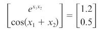
Use Newton-Raphson to find a solution towhere \(x_{1}\) and \(x_{2}\) are in radians.(a) Start with \(x_{1}(0)=1.0\) and \(x_{2}(0)=\) 0.5 and continue until (6.2.2) is satisfied with \(\varepsilon=0.005\).(b) Show that Newton-Raphson diverges for this example if \(x_{1}(0)=1.0\) and
Solve the following equations by the Newton-Raphson method:\[\begin{array}{r}2 x_{1}+x_{2}^{2}-8=0 \\x_{1}^{2}-x_{2}^{2}+x_{1} x_{2}-3=0\end{array}\]Start with an initial guess of \(x_{1}=1\) and \(x_{2}=1\).
The following nonlinear equations contain terms that are often found in the power flow equations:\[\begin{aligned}& f_{1}(x)=10 x_{1} \sin x_{2}+2=0 \\& f_{2}(x)=10\left(x_{1}ight)^{2}-10 x_{1} \cos x_{2}+1=0\end{aligned}\]Solve using the Newton-Raphson method starting with an initial guess of
Repeat Problem 6.25 except using x1(0)=0.25x1(0)=0.25 and x2(0)=0x2(0)=0 radians as an initial guess.Problem 6.25The following nonlinear equations contain terms that are often found in the power flow
For the Newton-Raphson method, the region of attraction (or basin of attraction) for a particular solution is the set of all initial guesses that converge to that solution. Usually initial guesses close to a particular solution will converge to that solution. However, for all but the simplest of
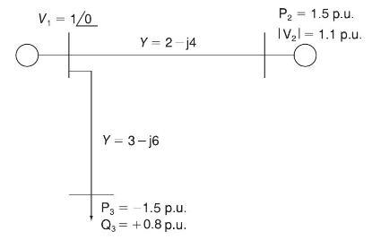
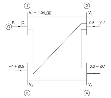
Consider the simplified electric power system shown in Figure 6.22 for which the power flow solution can be obtained without resorting to iterative techniques. (a) Compute the elements of the bus admittance matrix \(\boldsymbol{Y}_{\text {bus }}\) (b) Calculate the phase angle \(\delta_{2}\) by
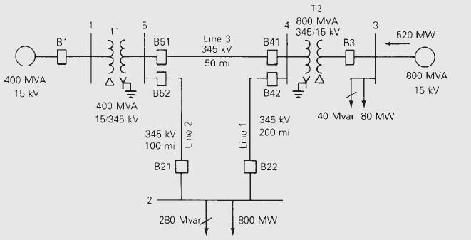
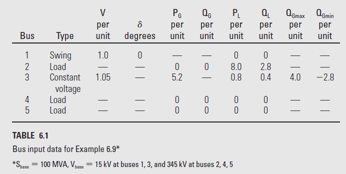
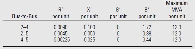
In Example 6.9, double the impedance on the line from bus 2 to bus 5 . Determine the new values for the second row of \(\boldsymbol{Y}_{\text {bus }}\). Verify your result using PowerWorld Simulator case Example 6_9.Example 6.9Figure 6.2 shows a single-line diagram of a five-bus power system. Input
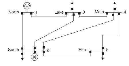
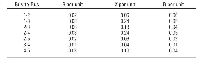
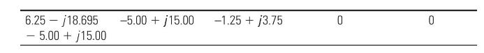
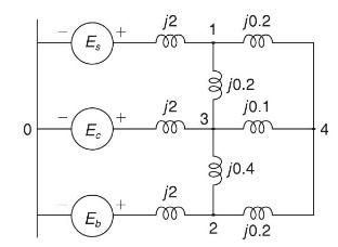
Determine the bus admittance matrix ( \(\boldsymbol{Y}_{\text {bus }}\) ) for the three-phase power system shown in Figure 6.23 with input data given in Table 6.11 and partial results in Table 6.12. Assume a three-phase 100 MVA per unit base.Table 6.11)Table 6.12) North South (1) 1 (1) 2 Lake 3
For the system from Problem 6.30, assume that a 75-Mvar shunt capacitance (three phase assuming one per unit bus voltage) is added at bus 4 . Calculate the new value of \(\mathrm{Y}_{44}\). 6.5}Problem 6.30Determine the bus admittance matrix ( \(\boldsymbol{Y}_{\text {bus }}\) ) for the three-phase
For a two-bus power system, a \(0.7+j 0.4 \) per unit load at bus 2 is supplied by a generator at bus 1 through a transmission line with series impedance of \(0.05+j 0.1 \) per unit. With bus 1 as the slack bus with a fixed per-unit voltage of \(1.0 \angle 0\), use the Gauss-Seidel method to
Repeat Problem 6.32 with the slack bus voltage changed to \(1.0 \angle 30^{\circ}\) per unit.Problem 6.32For a two-bus power system, a \(0.7+j 0.4 \) per unit load at bus 2 is supplied by a generator at bus 1 through a transmission line with series impedance of \(0.05+j 0.1 \) per unit. With bus 1
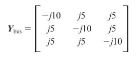
For the three-bus system whose \(\boldsymbol{Y}_{\text {bus }}\) is given, calculate the second iteration value of \(\mathrm{V}_{3}\) using the Gauss-Seidel method. Assume bus 1 as the slack (with \(V_{1}=1.0 / 0^{\circ}\) ), and buses 2 and 3 are load buses with a per-unit load of \(S_{2}=1+j 0.5
Repeat Problem 6.34 except assume the bus 1 (slack bus) voltage of \(V_{1}=\) \(1.05 \angle 0^{\circ}\).Problem 6.34For the three-bus system whose \(\boldsymbol{Y}_{\text {bus }}\) is given, calculate the second iteration value of \(\mathrm{V}_{3}\) using the Gauss-Seidel method. Assume bus 1 as
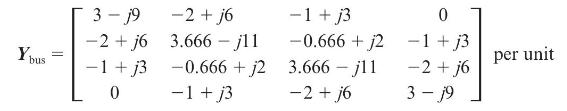
The bus admittance matrix for the power system shown in Figure 6.24 is given byWith the complex powers on load buses 2, 3, and 4 as shown in Figure 6.24, determine the value for \(\mathrm{V}_{2}\) that is produced by the first and second iterations of the Gauss-Seidel procedure. Choose the initial
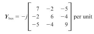
The bus admittance matrix of a three-bus power system is given bywith \(\mathrm{V}_{1}=1.0 \angle 0^{\circ}\) per unit; \(\mathrm{V}_{2}=1.0\) per unit; \(\mathrm{P}_{2}=60 \mathrm{MW} ; \mathrm{P}_{3}=-80 \mathrm{MW}\); \(\mathrm{Q}_{3}=-60\) Mvar (lagging) as a part of the power flow solution of
A generator bus (with a 1.0 per unit voltage) supplies a \(180 \mathrm{MW}, 60 \mathrm{Mvar}\) load through a lossless transmission line with per unit (100 MVA base) impedance of \(j 0.1 \) and no line charging. Starting with an initial voltage guess of \(1.0 / 0^{\circ}\), iterate until converged
Repeat Problem 6.38 except use an initial voltage guess of \(1.0 / 30^{\circ}\).Problem 6.38A generator bus (with a 1.0 per unit voltage) supplies a \(180 \mathrm{MW}, 60 \mathrm{Mvar}\) load through a lossless transmission line with per unit (100 MVA base) impedance of \(j 0.1 \) and no line
Repeat Problem 6.38 except use an initial voltage guess of \(0.25 \angle 0^{\circ}\).Problem 6.38A generator bus (with a 1.0 per unit voltage) supplies a \(180 \mathrm{MW}, 60 \mathrm{Mvar}\) load through a lossless transmission line with per unit (100 MVA base) impedance of \(j 0.1 \) and no line
Determine the initial Jacobian matrix for the power system described in Problem 6.34.Problem 6.34For the three-bus system whose \(\boldsymbol{Y}_{\text {bus }}\) is given, calculate the second iteration value of \(\mathrm{V}_{3}\) using the Gauss-Seidel method. Assume bus 1 as the slack (with
Use the Newton-Raphson power flow to solve the power system described in Problem 6.34. For convergence criteria, use a maximum power flow mismatch of 0.1 MVA.Problem 6.34For the three-bus system whose \(\boldsymbol{Y}_{\text {bus }}\) is given, calculate the second iteration value of
For a three-bus power system, assume bus 1 is the slack with a per unit voltage of 1.0∠0∘1.0∠0∘, bus 2 is a PQ bus with a per unit load of \(2.0+j 0.5 \), and bus 3 is a PV bus with 1.0 per unit generation and a 1.0 voltage setpoint. The per unit line impedances are \(j 0.1 \) between buses
Repeat Problem 6.43 except with the bus 2 real power load changed to 1.0 per unit.Problem 6.43or a three-bus power system, assume bus 1 is the slack with a per unit voltage of 1.0∠0∘1.0∠0∘, bus 2 is a PQ bus with a per unit load of 2.0+j0.52.0+j0.5, and bus 3 is a PV bus with 1.0 per unit
Load PowerWorld Simulator case Example 6_11; this case is set to perform a single iteration of the Newton-Raphson power flow each time Single Solution is selected. Verify that initially the Jacobian element \(J_{33}\) is 104.41. Then, give and verify the value of this element after each of the next
Load PowerWorld Simulator case Problem 6_46. Using a 100 MVA base, each of the three transmission lines have an impedance of \(0.05+j 0.1 \) p.u. There is a single \(180 \mathrm{MW}\) load at bus 3, while bus 2 is a PV bus with generation of \(80 \mathrm{MW}\) and a voltage setpoint of 1.0 p.u. Bus
As was mentioned in Section 6.4, if a generator's reactive power output reaches its limit, then it is modeled as though it were a PQ bus. Repeat Problem 6.46, except assume the generator at bus 2 is operating with its reactive power limited to a maximum of 50 Mvar. Then verify your solution by
Load PowerWorld Simulator case Problem 6_46. Plot the reactive power output of the generator at bus 2 as a function of its voltage setpoint value in 0.005 p.u. voltage steps over the range between its lower limit of -50 Mvar and its upper limit of 50 Mvar. To change the generator 2 voltage set
Open PowerWorld Simulator case Problem 6_49. This case is identical to Example 6.9, except that the transformer between buses 1 and 5 is now a tap-changing transformer with a tap range between 0.9 and 1.1 and a tap step size of 0.006 25 . The tap is on the high side of the transformer. As the tap
Use PowerWorld Simulator to determine the Mvar rating of the shunt capacitor bank in the Example 6_14 case that increases \(\mathrm{V}_{2}\) to 1.0 per unit. Also determine the effect of this capacitor bank on line loadings and the total real power losses (shown immediately below bus 2 on the
Use PowerWorld Simulator to modify the Example 6_9 case by inserting a second line between bus 2 and bus 5. Give the new line a circuit identifier of " 2 " to distinguish it from the existing line. The line parameters of the added line should be identical to those of the existing lines 2 to 5 .
Open PowerWorld Simulator case Problem 6_52. Open the \(69 \mathrm{kV}\) line between buses REDBUD69 and PEACH69 (shown towards the bottom of the oneline). With the line open, determine the amount of Mvar (to the nearest 1 Mvar) needed from the REDBUD69 capacitor bank to correct the REDBUD69
Open PowerWorld Simulator case Problem 6_53. Plot the variation in the total system real power losses as the generation at bus PEAR 138 is varied in \(20 \mathrm{MW}\) blocks between \(0 \mathrm{MW}\) and \(400 \mathrm{MW}\). What value of PEAR 138 generation minimizes the total system losses?
Repeat Problem 6.53, except first remove the \(69 \mathrm{kV}\) line between LOCUST69 and PEAR69.Problem 6.53Open PowerWorld Simulator case Problem 6_53. Plot the variation in the total system real power losses as the generation at bus PEAR 138 is varied in \(20 \mathrm{MW}\) blocks between \(0
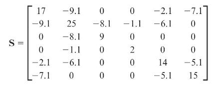
Using the compact storage technique described in Section 6.8, determine the vectors DIAG, OFFDIAG, COL, and ROW for the following matrix: S= 17 -9.1 25 0 -8.1 0 -1.1 -6.1 -9.1 -2.1 -7.1 0 0 -8.1 9 0 0 0 0 -1.1 0 2 0 0 -2.1 -7.1 -6.1 0 0 0 0 14 -5.1 0 -5.1 15
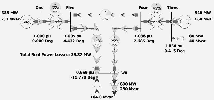
For the triangular factorization of the corresponding \(\boldsymbol{Y}_{\text {bus }}\), number the nodes of the graph shown in Figure 6.9 in an optimal order.Figure 6.9 385 MW -37 Mvar slack One 65% Five MVA 1.000 pu 0.000 Deg 1.005 pu -4.432 Deg Total Real Power Losses: 25.37 MW 44% MVA 0.959 pu-
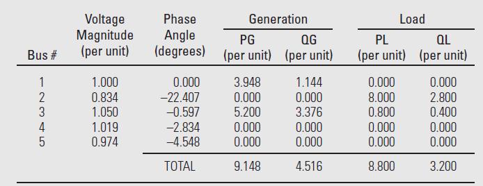
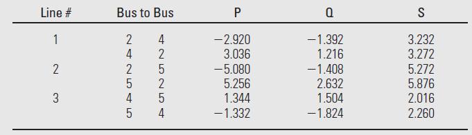
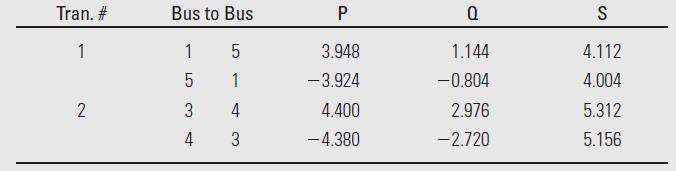
Compare the angles and line flows between the Example 6_17 case and results shown in Tables 6.6, 6.7, and 6.8.Table 6.6Table 6.7Table 6.8Example 6_17Determine the dc power flow solution for the five bus system from Example 6.9.Example 6.9Figure 6.2 shows a single-line diagram of a five-bus power
Redo Example 6.17 with the assumption that the per-unit reactance on the line between buses 2 and 5 is changed from 0.05 to 0.03.Example 6.17Determine the dc power flow solution for the five bus system from Example 6.9.Example 6.9Figure 6.2 shows a single-line diagram of a five-bus power system.
Open PowerWorld Simulator case Problem 6_59, which models a seven-bus system using the de power flow approximation. Bus 7 is the system slack. The real power generation/load at each bus is as shown, while the per-unit reactance of each of the lines (on a 100 MVA base) is as shown in yellow on the
Using the PowerWorld Simulator case from Problem 6.59, if the rating on the line between buses 1 and 2 is \(150 \mathrm{MW}\), the current flow is \(101 \mathrm{MW}\) (from bus 1 to bus 3 ), and the bus 1 generation is \(160 \mathrm{MW}\), analytically determine the amount this generation can
PowerWorld Simulator cases Problem 6_61_PQ and 6_61_PV model a sevenbus power system in which the generation at bus 4 is modeled as a Type 1 or 2 wind turbine in the first case and as a Type 3 or 4 wind turbine in the second. A shunt capacitor is used to make the net reactive power injection at the
The fuel-cost curves for two generators are given as follows:\[\begin{aligned}& \mathrm{C}_{1}\left(\mathrm{P}_{1}ight)=600+18 \cdot \mathrm{P}_{1}+0.04 \cdot\left(\mathrm{P}_{1}ight)^{2} \\& \mathrm{C}_{2}\left(\mathrm{P}_{2}ight)=700+20 \cdot \mathrm{P}_{2}+0.03
Rework Problem 6.62, except assume that the limit outputs are subject to the following inequality constraints:\[\begin{aligned}& 200 \leq \mathrm{P}_{1} \leq 800 \mathrm{MW} \\& 100 \leq \mathrm{P}_{2} \leq 400 \mathrm{MW}\end{aligned}\]Problem 6.62The fuel-cost curves for two generators are given
Rework Problem 6.62, except assume the \(1000 \mathrm{MW}\) value also includes losses, and the penalty factor for the first unit is 1.0 and for the second unit 0.95.Problem 6.62The fuel-cost curves for two generators are given as follows:\[\begin{aligned}&
The fuel-cost curves for a two-generator power system are given as follows:\[\begin{aligned}& \mathrm{C}_{1}\left(\mathrm{P}_{1}ight)=600+15 \cdot \mathrm{P}_{1}+0.05 \cdot\left(\mathrm{P}_{1}ight)^{2} \\& \mathrm{C}_{2}\left(\mathrm{P}_{2}ight)=700+20 \cdot \mathrm{P}_{2}+0.04
Expand the summations in (6.12.14) for \(N=2\), and verify the formula for \(\partial \mathrm{P}_{\mathrm{L}} / \partial \mathrm{P}_{i}\) given by (6.12.15). Assume \(\mathrm{B}_{i j}=\mathrm{B}_{j i}\).
Given two generating units with their respective variable operating costs as\[\begin{array}{ll}\mathrm{C}_{1}=0.01 \mathrm{P}_{\mathrm{G} 1}^{2}+2 \mathrm{P}_{\mathrm{G} 1}+100 \$ / \mathrm{hr} & \text { for } 25 \leq \mathrm{P}_{\mathrm{G} 1} \leq 150 \mathrm{MW} \\\mathrm{C}_{2}=0.004
Resolve Example 6.20, except with the generation at bus 2 set to a fixed value (i.e., modeled as off of Automatic Generation Control). Plot the variation in the total hourly cost as the generation at bus 2 is varied between 1000 and 200 MW in 5 MW steps, resolving the economic dispatch at each
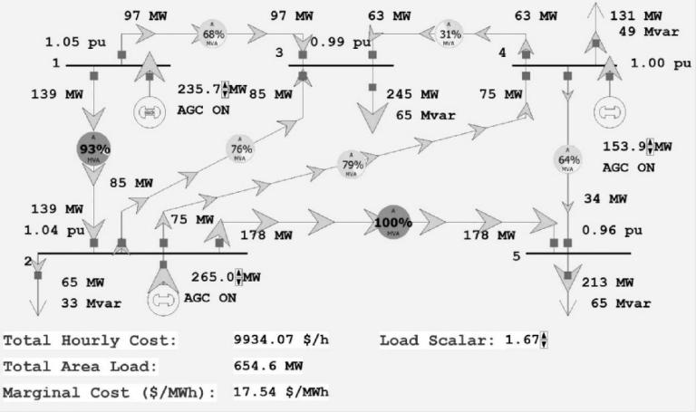
Using PowerWorld case Example 6_22 with the Load Scalar equal to 1.0, determine the generation dispatch that minimizes system losses. Manually vary the generation at buses 2 and 4 until their loss sensitivity values are zero. Compare the operating cost between this solution and the Example 6_22
Repeat Problem 6.69, except with the Load Scalar equal to 1.4.Problem 6.69Using PowerWorld case Example 6_22 with the Load Scalar equal to 1.0, determine the generation dispatch that minimizes system losses. Manually vary the generation at buses 2 and 4 until their loss sensitivity values are zero.
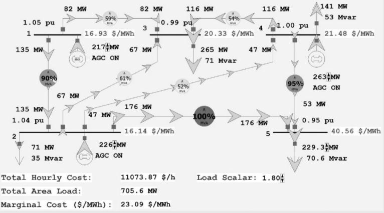
Using LP OPF with PowerWorld Simulator case Example 6_23, plot the variation in the bus 5 marginal price as the Load Scalar is increased from 1.0 in steps of 0.02. What is the maximum possible load scalar without overloading any transmission line? Why is it impossible to operate without violations
Load PowerWorld Simulator case Problem 6_72. This case models a slightly modified, lossless version of the 37-bus case from Example 6.13 with generator cost information, but also with the transformer between buses PEAR138 and PEAR69 open. When the case is loaded, the "Total Cost" field shows the
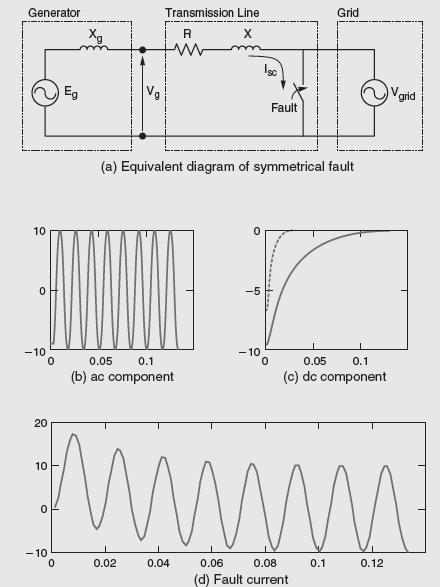
The asymmetrical short-circuit current in series \(\mathrm{R}-\mathrm{L}\) circuit for a simulated solid or "bolted fault" can be considered as a combination of symmetrical (ac) component that is a ____________, and dc-offset current that decays ____________ and depends on ____________.
Even though the fault current is not symmetrical and not strictly periodic, the rms asymmetrical fault current is computed as the rms ac fault current times an "asymmetry factor," which is a function of ____________.
The amplitude of the sinusoidal symmetrical ac component of the three-phase short-circuit current of an unloaded synchronous machine decreases from a high initial value to a lower steady-state value, going through the stages of ____________ and ____________ periods.
The duration of subtransient fault current is dictated by time ____________ constant and that of transient fault current is dictated by time ____________ constant.
The reactance that plays a role under steady-state operation of a synchronous machine is called ____________.
The dc-offset component of the three-phase short-circuit current of an unloaded synchronous machine is different in the three phases and its exponential decay is dictated by ____________.
Generally, in power-system short-circuit studies, for calculating subtransient fault currents, transformers are represented by their ____________ transmission lines by their equivalent ____________ and synchronous machines by ____________ behind their subtransient reactances.
In power-system fault studies, all nonrotating impedance loads are usually neglected.(a) True(b) False
Can superposition be applied in power-system short-circuit studies for calculating fault currents?(a) Yes(b) No
Before proceeding with per-unit fault current calculations, based on the single-line diagram of the power system, a positive-sequence equivalent circuit is set up on a chosen base system.(a) True(b) False
The inverse of the bus-admittance matrix is called a ____________ matrix.
For a power system, modeled by its positive-sequence network, both busadmittance matrix and bus-impedance matrix are symmetric.(a) True(b) False
The bus-impedance equivalent circuit can be represented in the form of a "rake" with the diagonal elements, which are ____________ and the non-diagonal (off-diagonal) elements, which are ____________.
A circuit breaker is designed to extinguish the arc by ____________.
Power-circuit breakers are intended for service in the ac circuit above ____________ V.
In circuit breakers, besides air or vacuum, what gaseous medium, in which the arc is elongated, is used?
Oil can be used as a medium to extinguish the arc in circuit breakers.(a) True(b) False
Besides a blast of air/gas, the arc in a circuit breaker can be elongated by ____________.
For distribution systems, standard reclosers are equipped for two or more reclosures, whereas multiple-shot reclosing in EHV systems is not a standard practice.(a) True(b) False
Breakers of the \(115 \mathrm{kV}\) class and higher have a voltage range factor \(\mathrm{K}=\) ____________, such that their symmetrical interrupting current capability remains constant.
A typical fusible link metal in fuses is ____________, and a typical filler material is
The melting and clearing time of a current-limiting fuse is usually specified by a ____________ curve.
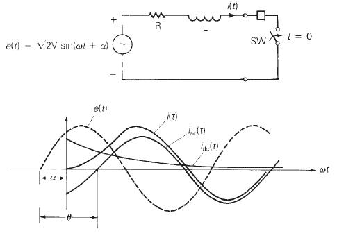
In the circuit of Figure 7.1, \(\mathrm{V}=277\) volts, \(\mathrm{L}=2 \mathrm{mH}, \mathrm{R}=0.4 \Omega\), and \(\omega=2 \pi 60 \mathrm{rad} / \mathrm{s}\). Determine (a) the rms symmetrical fault current; (b) the rms asymmetrical fault current at the instant the switch closes, assuming
Repeat Example 7.1 with \(\mathrm{V}=4 \mathrm{kV}, \mathrm{X}=2 \Omega\), and \(\mathrm{R}=1 \Omega\)Example 7.1A bolted short circuit occurs in the series R–L circuit of Figure 7.1 with V = 20 kV, X = 8 V, R = 0.8 V, and with maximum dc offset. The circuit breaker opens 3 cycles after fault
In the circuit of Figure 7.1, let \(\mathrm{R}=0.125 \Omega ., \mathrm{L}=10 \mathrm{mH}\), and the source voltage is \(e(\mathrm{t})=151 \sin (377 \mathrm{t}+\alpha) \mathrm{V}\). Determine the current response after closing the switch for the following cases:(a) no dc offset or(b) maximum dc
Consider the expression for \(i(t)\) given by\[i(t)=\sqrt{2} \mathrm{I}_{\mathrm{rms}}\left[\sin \left(\omega t-\theta_{z}ight)+\sin \theta_{z} \cdot e^{-(\omega R / X) t}ight]\]where \(\theta_{z}=\tan ^{-1}(\omega L / R)\).(a) For \((\mathrm{X} / \mathrm{R})\) equal to zero and infinity, plot
If the source impedance at a \(13.2-\mathrm{kV}\) distribution substation bus is \((0.5+\) j1.5) \(\Omega\) per phase, compute the rms and maximum peak instantaneous value of the fault current for a balanced three-phase fault. For the system \((\mathrm{X} / \mathrm{R})\) ratio of 3.0, the
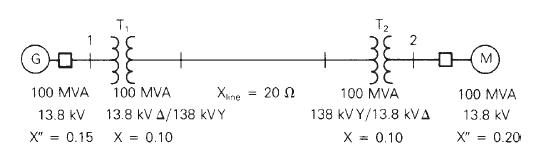
A 1000-MVA, \(20-\mathrm{kV}, 60-\mathrm{Hz}\), three-phase generator is connected through a \(1000-\mathrm{MVA}, 20-\mathrm{kV}, \Delta / 345-\mathrm{kV}\), Y transformer to a \(345-\mathrm{kV}\) circuit breaker and a \(345-\mathrm{kV}\) transmission line. The generator reactances are
For Problem 7.6, determine(a) the instantaneous symmetrical fault current in kA in phase \(a\) of the generator as a function of time, assuming maximum dc offset occurs in this generator phase, and(b) the maximum \(\mathrm{dc}\) offset current in \(\mathrm{kA}\) as a function of time that can occur
A 300-MVA, 13.8-kV, three-phase, \(60-\mathrm{Hz}\), Y-connected synchronous generator is adjusted to produce rated voltage on open circuit. A balanced three-phase fault is applied to the terminals at \(t=0\). After analyzing the raw data, the symmetrical transient current is obtained
Two identical synchronous machines, each rated \(60 \mathrm{MVA}\) and \(15 \mathrm{kV}\) with a subtransient reactance of 0.1 p.u., are connected through a line of reactance 0.1 p.u. on the base of the machine rating. One machine is acting as a synchronous generator, while the other is working as
Recalculate the subtransient current through the breaker in Problem 7.6 if the generator is initially delivering rated MVA at 0.80 p.f. lagging and at rated terminal voltage.Problem 7.6A 1000-MVA, \(20-\mathrm{kV}, 60-\mathrm{Hz}\), three-phase generator is connected through a \(1000-\mathrm{MVA},
Solve Example 7.3 parts (a) and (c) without using the superposition principle. First calculate the internal machine voltages \(E_{g}^{\prime \prime}\) and \(E_{m}^{\prime \prime}\) using the prefault load current. Then determine the subtransient fault, generator, and motor currents directly from
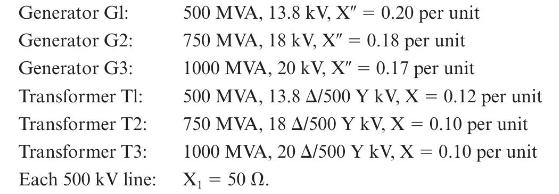
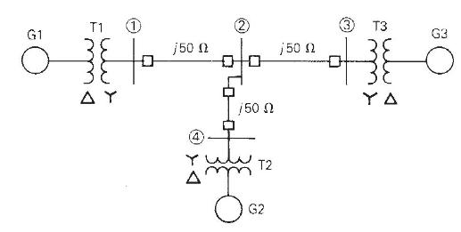
Equipment ratings for the four-bus power system shown in Figure 7.14 are as follows: A three-phase short circuit occurs at bus 1, where the prefault voltage is \(525 \mathrm{kV}\). Prefault load current is neglected. Draw the positive-sequence reactance diagram in per unit on a
For the power system given in Problem 7.12, a three-phase short circuit occurs at bus 2, where the prefault voltage is \(525 \mathrm{kV}\). Prefault load current is neglected. Determine the(a) Thévenin equivalent at the fault,(b) subtransient fault current in per unit and in kA rms, and(c)
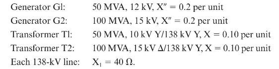
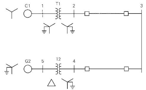
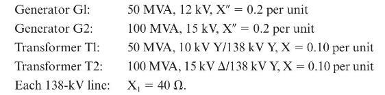
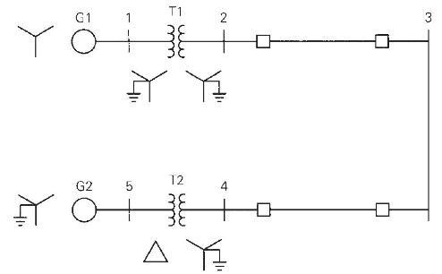
Equipment ratings for the five-bus power system shown in Figure 7.15 are as follows:A three-phase short circuit occurs at bus 5, where the prefault voltage is 15kV15kV. Prefault load current is neglected.(a) Draw the positive-sequence reactance diagram in per unit on a
For the power system given in Problem 7.14, a three-phase short circuit occurs at bus 4 , where the prefault voltage is \(138 \mathrm{kV}\). Prefault load current is neglected. Determine(a) the Thévenin equivalent at the fault,(b) the subtransient fault current in per unit and in kA rms, and(c)
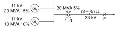
In the system shown in Figure 7.16, a three-phase short circuit occurs at point F. Assume that prefault currents are zero and that the generators are operating at rated voltage. Determine the fault current. 11 KV 20 MVA 15% 11 kV 10 MVA 10% G (G) 30 MVA 5% 1:3 (3 + j5) 33 kV * F LL
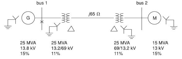
A three-phase short circuit occurs at the generator bus (bus 1) for the system shown in Figure 7.17. Neglecting prefault currents and assuming that the generator is operating at its rated voltage, determine the subtransient fault current using superposition. G bus 1 25 MVA 13.8 kV 15% A 25 MVA
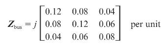
(a) The bus impedance matrix for a three-bus power system iswhere subtransient reactances were used to compute \(\boldsymbol{Z}_{\text {bus }}\). Prefault voltage is 1.0 per unit and prefault current is neglected. (a) Draw the bus impedance matrix equivalent circuit (rake equivalent). Identify the
Determine \(\boldsymbol{Y}_{\text {bus }}\) in per unit for the circuit in Problem 7.12. Then invert \(\boldsymbol{Y}_{\text {bus }}\) to obtain \(\boldsymbol{Z}_{\text {bus }}\).Problem 7.12Equipment ratings for the four-bus power system shown in Figure 7.14 are as follows: A three-phase short
Determine \(\boldsymbol{Y}_{\text {bus }}\) in per unit for the circuit in Problem 7.14. Then invert \(\boldsymbol{Y}_{\text {bus }}\) to obtain \(\boldsymbol{Z}_{\text {bus }}\).Problem 7.14Equipment ratings for the five-bus power system shown in Figure 7.15 are as follows:A three-phase short
Figure 7.18 shows a system reactance diagram. (a) Draw the admittance diagram for the system by using source transformations. (b) Find the bus admittance matrix \(\boldsymbol{Y}_{\text {bus }}\) (c) Find the bus impedance \(\boldsymbol{Z}_{\text {bus }}\) matrix by inverting \(\boldsymbol{Y}_{\text
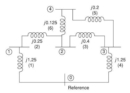
For the network shown in Figure 7.19, impedances labeled 1 through 6 are in per unit. (a) Determine \(\boldsymbol{Y}_{\text {bus }}\), preserving all buses. (b) Using MATLAB or a similar computer program, invert \(\boldsymbol{Y}_{\text {bus }}\) to obtain \(\boldsymbol{Z}_{\text {bus }}\). 1 m oooo
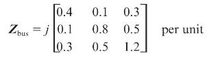
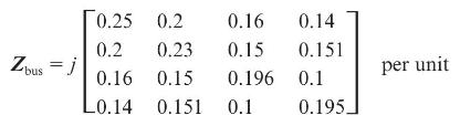
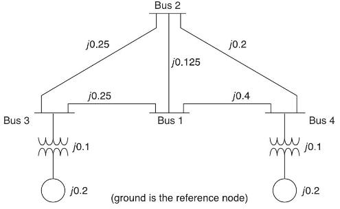
A single-line diagram of a four-bus system is shown in Figure 7.20, for which \(\boldsymbol{Z}_{\text {bus }}\) is given below:Let a three-phase fault occur at bus 2 of the network.(a) Calculate the initial symmetrical rms current in the fault.(b) Determine the voltages during the fault at buses 1,
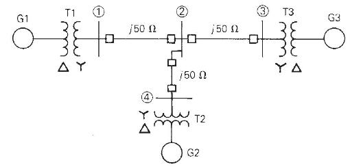
PowerWorld Simulator case Problem 7_24 models the system shown in Figure 7.14 with all data on a 1000 MVA base. Using PowerWorld Simulator, determine the current supplied by each generator and the per-unit bus voltage magnitudes at each bus for a fault at bus 3 .Figure 7.14 G1 T1 1 j50 ( 150 T T2

Showing 3400 - 3500 of 5433

First
28
29
30
31
32
33
34
35
36
37
38
39
40
41
42
Last

Step by Step Answers

Services

Sitemap
Fun
Definitions
Become Tutor
Used Textbooks
Study Help Categories
Recent Questions
Expert Questions
Campus Wear
Sell Your Books

Company Info

Security
Copyrights
Privacy Policy
Terms & Conditions
SolutionInn Fee
Scholarship
Online Quiz
Give Feedback, Get Rewards

Get In Touch

About Us
Contact Us
Career
Jobs
FAQ
Student Discount
Campus Ambassador

Secure Payment

Download Our App

© 2026 SolutionInn. All Rights Reserved