New Semester Started Get 50% OFF Study Help! --h --m --s Claim Now

Question Answers

Textbooks

Find textbooks, questions and answers

Oops, something went wrong!

Change your search query and then try again

Result Not Found

Books FREE
Study Help
Tutors
AI Study Planner NEW
Sell Books

Search
Sign In
Register

study help
computer science
systems analysis design

The Analysis And Design Of Linear Circuits 10th Edition Roland E. Thomas, Albert J. Rosa, Gregory J. Toussaint - Solutions

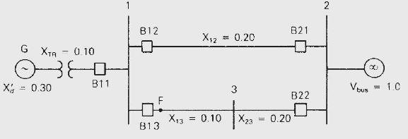
Open PowerWorld Simulator case Problem 11_20. This case models the Example 11.4 system with damping at the bus 1 generator, and with a line fault midway between buses 1 and 2 . The fault is cleared by opening the line. Determine the critical clearing time for this fault.Example 11.4The synchronous
Open PowerWorld Simulator case Problem 11_21. This case models the Example 11.4 system with damping at the bus 1 generator, and with a line fault midway between buses 2 and 3. The fault is cleared by opening the line. Determine the critical clearing time (to the nearest 0.01 second) for this
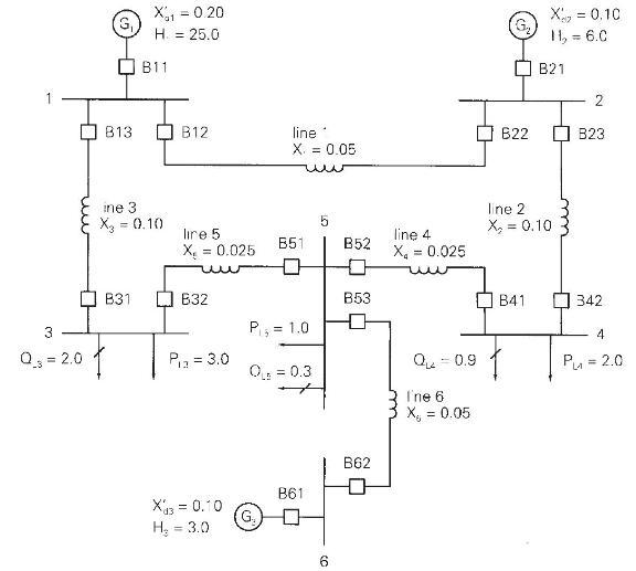
Consider the six-bus power system shown in Figure 11.29, where all data are given in per-unit on a common system base. All resistances as well as transmission-line capacitances are neglected. (a) Determine the \(6 \times 6\) per-unit bus admittance matrix \(\boldsymbol{Y}_{\text {bus }}\) suitable
Modify the matrices Y11,Y12Y11,Y12, and Y22Y22 determined in Problem 11.22 for(a) the case when circuit breakers B32 and B51 open to remove line 3-5; and(b) the case when the load PL3+jQL3PL3+jQL3 is removed.Problem 11.22Consider the six-bus power system shown in Figure 11.29, where all data are
Open PowerWorld Simulator case Problem 11_24, which models the Example 6.9 with transient stability data added for the generators. Determine the critical clearing time (to the nearest 0.01 second) for a fault on the line between buses 4 and 5 at the bus 4 end which is cleared by opening the line. 3
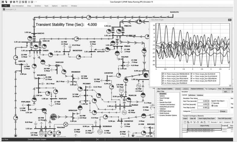
With PowerWorld Simulator using the Example 11_9 case determine the critical clearing time (to the closest 0.01 second) for a transmission line fault on the transmission line between bus 44 (PEACH69) and bus 14 (REDBUD69), with the fault occurring near bus 44.Example 11_9PowerWorld Simulator case
PowerWorld Simulator case Problem 11_26 duplicates Example 11.10, except with the synchronous generator initially supplying \(75 \mathrm{MW}\) at unity power factor to the infinite bus.(a) Derive the initial values for \(\delta, \mathrm{E}_{q}^{\prime}, \mathrm{E}_{d}^{\prime}\) and \(\mathrm{E}_{f
PowerWorld Simulator case Problem 11_27 duplicates the system from Problem 11.24, except the generators are modeled using a two-axis model, with the same \(\mathrm{X}_{d}^{\prime}\) and \(\mathrm{H}\) parameters as are in Problem 11.24. Compare the critical clearing time between this case and the
PowerWorld Simulator case Problem 11_28 duplicates Example 11.11 except the wind turbine generator is set so it is initially supplying \(100 \mathrm{MW}\) to the infinite bus at unity power factor.(a) Use the induction machine equations to verify the initial conditions of \(\mathrm{S}=-0.0129,
Redo Example 11.12 with the assumption the generator is supplying \(100+j 10\) MVA to the infinite bus.Example 11.12For the system from Example 11.3, assume the synchronous generator is replaced with an induction generator and shunt capacitor in order to represent a wind farm with the same initial
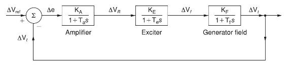
The block-diagram representation of a closed-loop automatic regulating system, in which generator voltage control is accomplished by controlling the exciter voltage, is shown in Figure 12.14. \(\mathrm{T}_{\mathrm{a}}, \mathrm{T}_{\mathrm{e}}\), and \(\mathrm{T}_{\mathrm{f}}\) are the time
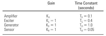
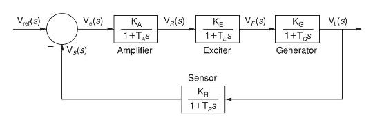
The Automatic Voltage Regulator (AVR) system of a generator is represented by the simplified block diagram shown in Figure 12.15, in which the sensor is modeled by a simple first-order transfer function. The voltage is sensed through a voltage transformer and then rectified through a bridge
Open PowerWorld Simulator case Problem 12_3. This case models the system from Example 12.1 except with the rate feedback gain constant, \(\mathrm{K}_{\mathrm{f}}\), has been set to zero and the simulation end time was increased to 30 seconds. Without rate feedback the system voltage response will
An area of an interconnected \(60-\mathrm{Hz}\) power system has three turbinegenerator units rated 200,300, and 500 MVA. The regulation constants of the units are \(0.03,0.04\), and 0.05 per unit, respectively, based on their ratings. Each unit is initially operating at one-half its own rating
Each unit in Problem 12.5 is initially operating at one-half its own rating when the load suddenly increases by 100 MW. Determine(a) the steadystate decrease in area frequency, and(b) the MW increase in mechanical power output of each turbine. Assume that the reference power setting of each
Each unit in Problem 12.5 is initially operating at one-half its own rating when the frequency increases by 0.005 per unit. Determine the MW decrease of each unit. The reference power setting of each turbinegovernor is fixed. Neglect losses and the dependence of load on frequency.Problem 12.5An
Repeat Problem 12.7 if the frequency decreases by 0.005 per unit. Determine the MW increase of each unit.Problem 12.7Each unit in Problem 12.5 is initially operating at one-half its own rating when the frequency increases by 0.005 per unit. Determine the MW decrease of each unit. The reference
An interconnected \(60-\mathrm{Hz}\) power system consisting of one area has two turbine-generator units, rated 500 and \(750 \mathrm{MVA}\), with regulation constants of 0.04 and 0.06 per unit, respectively, based on their respective ratings. When each unit carries a 300-MVA steady-state load, let
Open PowerWorld Simulator case Problem 12_10. The case models the system from Example 12.4 except 1) the load increases is a \(50 \%\) rise at bus 6 for a total increase of \(250 \mathrm{MW}\) (from \(500 \mathrm{MW}\) to \(750 \mathrm{MW}\) ), 2) the value of \(\mathrm{R}\) for generator 1 is
Open PowerWorld Simulator case Problem 12_11, which includes a transient stability representation of the system. Each generator is modeled using a two-axis machine model, an IEEE Type 1 exciter and a TGOV 1 governor with \(\mathrm{R}=0.04\) per unit (a summary of the generator models is available
Repeat Problem 12.11 except first double the \(\mathrm{H}\) value for each of the machines. This can be most easily accomplished by selecting Stability Case Info, Transient Stability Case Summary to view the summary form. Right click on the line corresponding to the Machine Model class, and then
For a large, \(60 \mathrm{~Hz}\), interconnected electrical system assume that following the loss of two \(1400 \mathrm{MW}\) generators (for a total generation loss of \(2800 \mathrm{MW}\) ) the change in frequency is \(-0.12 \mathrm{~Hz}\). If all the on-line generators that are available to
A \(60-\mathrm{Hz}\) power system consists of two interconnected areas. Area 1 has \(1200 \mathrm{MW}\) of generation and an area frequency response characteristic \(\beta_{1}=400 \mathrm{MW} / \mathrm{Hz}\). Area 2 has \(1800 \mathrm{MW}\) of generation and \(\beta_{2}=\) \(600 \mathrm{MW} /
Repeat Problem 12.14 if \(\mathrm{LFC}\) is employed in area 2 alone. The area 2 frequency bias coefficient is set at \(\mathrm{B}_{f 2}=\beta_{2}=600 \mathrm{MW} / \mathrm{Hz}\). Assume that LFC in area 1 is inoperative due to a computer failure.Problem 12.14A \(60-\mathrm{Hz}\) power system
Repeat Problem 12.14 if \(\mathrm{LFC}\) is employed in both areas. The frequency bias coefficients are \(\mathrm{B}_{f 1}=\beta_{1}=400 \mathrm{MW} / \mathrm{Hz}\) and \(\mathrm{B}_{f 2}=\beta_{2}=600 \mathrm{MW} / \mathrm{Hz}\).Problem 12.14A \(60-\mathrm{Hz}\) power system consists of two
Rework Problems 12.15 through 12.16 when the load in area 2 suddenly decreases by \(300 \mathrm{MW}\). The load in area 1 does not change.Problem 12.15Repeat Problem 12.14 if \(\mathrm{LFC}\) is employed in area 2 alone. The area 2 frequency bias coefficient is set at \(\mathrm{B}_{f
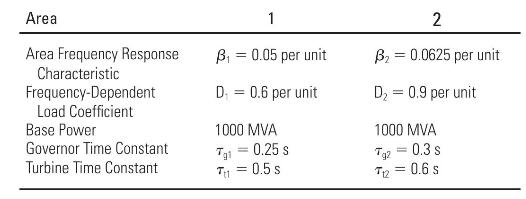
On a 1000-MVA common base, a two-area system interconnected by a tie line has the following parameters:The two areas are operating in parallel at the nominal frequency of \(60 \mathrm{~Hz}\). The areas are initially operating in steady state with each area supplying 1000 MW when a sudden load
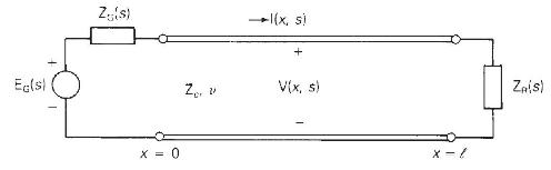
From the results of Example 13.2, plot the voltage and current profiles along the line at times \(\tau / 2, \tau\), and \(2 \tau\). That is, plot \(v(x, \tau / 2)\) and \(i(x, \tau / 2)\) versus \(x\) for \(0 \leqslant x \leqslant 1\); then plot \(v(x, \tau), i(x, x), v(x, 2 \tau)\), and \(i(x, 2
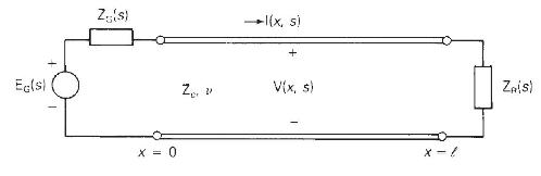
Rework Example 13.2 if the source voltage at the sending end is a ramp, \(e_{\mathrm{G}}(t)=\mathrm{E} u_{-2} \mathrm{M}=\mathrm{E} t u_{-1}(t)\), with \(\mathrm{Z}_{\mathrm{G}}=2 \mathrm{Z}_{c}\).Example 13.2The receiving end is open. The source voltage at the sending end is a step
Referring to the single-phase two-wire lossless line shown in Figure 13.3, the receiving end is terminated by an inductor with \(2 \mathrm{~L}_{\mathrm{R}}\) henries. The source voltage at the sending end is a step, \(e_{\mathrm{G}}(t)=\mathrm{E} u_{-1}(t)\) with \(\mathrm{Z}_{\mathrm{G}}=Z_{c}\).
Rework Problem 13.3 if \(Z_{\mathrm{R}}=Z_{c}\) at the receiving end and the source voltage at the sending end is \(e_{\mathrm{G}}(t)=\mathrm{E} u_{-1}(t)\), with an inductive source impedance \(\mathrm{Z}_{\mathrm{G}}(s)=s 2 \mathrm{~L}_{\mathrm{G}}\). Both the line and source inductor are
Rework Example 13.4 with \(\mathrm{Z}_{\mathrm{R}}=5 \mathrm{Z}_{c}\) and \(\mathrm{Z}_{\mathrm{G}}=\mathrm{Z}_{c} / 3\).Example 13.4At the receiving end, \(\mathrm{Z}_{\mathrm{R}}=\mathrm{Z}_{c} / 3\). At the sending end, \(e_{\mathrm{G}}(t)=\mathrm{Eu}_{-1}(t)\) and \(\mathrm{Z}_{\mathrm{G}}=2
The single-phase, two-wire lossless line in Figure 13.3 has a series inductance \(\mathrm{L}=(1 / 3) \times 10^{-6} \mathrm{H} / \mathrm{m}\), a shunt capacitance \(\mathrm{C}=(1 / 3) \times 10^{-10} \mathrm{~F} / \mathrm{m}\), and a \(50-\mathrm{km}\) line length. The source voltage at the sending
The single-phase, two-wire lossless line in Figure 13.3 has a series inductance \(\mathrm{L}=2 \times 10^{-6} \mathrm{H} / \mathrm{m}\), a shunt capacitance \(\mathrm{C}=1.25 \times 10^{-11} \mathrm{~F} / \mathrm{m}\), and a \(100-\mathrm{km}\) line length. The source voltage at the sending end is
The single-phase, two-wire lossless line in Figure 13.3 has a series inductance \(\mathrm{L}=0.999 \times 10^{-6} \mathrm{H} / \mathrm{m}\), a shunt capacitance \(\mathrm{C}=1.112 \times 10^{-11} \mathrm{~F} / \mathrm{m}\), and a \(60-\mathrm{km}\) line length. The source voltage at the sending end
Draw the Bewley lattice diagram for Problem 13.5.Problem 13.5Rework Example 13.4 with \(\mathrm{Z}_{\mathrm{R}}=5 \mathrm{Z}_{c}\) and \(\mathrm{Z}_{\mathrm{G}}=\mathrm{Z}_{c} / 3\).Example 13.4At the receiving end, \(\mathrm{Z}_{\mathrm{R}}=\mathrm{Z}_{c} / 3\). At the sending end,
Rework Problem 13.9 if the source voltage is a pulse of magnitude \(\mathrm{E}\) and duration \(\tau / 10\); that is, \(e_{\mathrm{G}}(t)=\mathrm{E}\left[u_{-1}(t)-u_{-1}(t-\tau / 10)ight]\). \(\mathrm{Z}_{\mathrm{R}}=5 \mathrm{Z}_{c}\) and \(\mathrm{Z}_{\mathrm{G}}=\) \(\mathrm{Z}_{c} / 3\) are
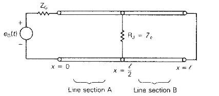
As shown in Figure 13.32, a single-phase two-wire lossless line with \(Z_{c}=\) \(400 \Omega, v=3 \times 10^{8} \mathrm{~m} / \mathrm{s}\), and \(1=100 \mathrm{~km}\) has a \(400-\Omega\) resistor, denoted \(\mathrm{R}_{\mathrm{J}}\), installed across the center of the line, thereby dividing the
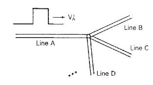
The junction of four single-phase two-wire lossless lines, denoted A, B, \(\mathrm{C}\), and \(\mathrm{D}\), is shown in Figure 13.13. Consider a voltage wave \(v_{\mathrm{A}}^{+}\)arriving at the junction from line A. Using (13.3.8) and (13.3.9), determine the voltage reflection coefficient
Referring to Figure 13.3, the source voltage at the sending end is a step \(e_{\mathrm{G}}(t)=\mathrm{Eu}_{-1}(t)\) with an inductive source impedance \(\mathrm{Z}_{\mathrm{G}}(s)=s \mathrm{~L}_{\mathrm{G}}\), where \(\mathrm{L}_{\mathrm{G}} / \mathrm{Z}_{c}=\tau / 3\). At the receiving end,
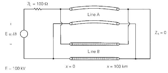
As shown in Figure 13.33, two identical, single-phase, two-wire, lossless lines are connected in parallel at both the sending and receiving ends. Each line has a \(400-\Omega\) characteristic impedance, \(3 \times 10^{8} \mathrm{~m} / \mathrm{s}\) velocity of propagation, and \(100-\mathrm{km}\)
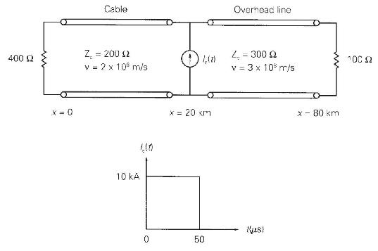
As shown in Figure 13.34, an ideal current source consisting of a 10-kA pulse with \(50-\mu\) s duration is applied to the junction of a single-phase, lossless cable and a single-phase, lossless overhead line. The cable has a \(200-\Omega\) characteristic impedance, \(2 \times 10^{8} \mathrm{~m} /
For the circuit given in Problem 13.3, replace the circuit elements by their discrete-time equivalent circuits and write nodal equations in a form suitable for computer solution of the sending-end and receiving-end voltages. Give equations for all dependent sources. Assume \(\mathrm{E}=1000
Repeat Problem 13.18 for the circuit given in Problem 13.13. Assume \(\Delta t=0.03333 \mathrm{~ms}\).Problem 13.18For the circuit given in Problem 13.3, replace the circuit elements by their discrete-time equivalent circuits and write nodal equations in a form suitable for computer solution of the
For the circuit given in Problem 13.7, replace the circuit elements by their discrete-time equivalent circuits. Use \(\Delta t=100 \mu \mathrm{s}=1 \times 10^{-4} \mathrm{~s}\). Determine and show all resistance values on the discrete-time circuit. Write nodal equations for the discrete-time
For the circuit given in Problem 13.8, replace the circuit elements by their discrete-time equivalent circuits. Use \(\Delta t=50 \mu \mathrm{s}=5 \times 10^{-5} \mathrm{~s}\) and \(\mathrm{E}=\) \(100 \mathrm{kV}\). Determine and show all resistance values on the discrete-time circuit. Write nodal
Rework Problem 13.18 for a lossy line with a constant series resistance \(\mathrm{R}=0.3 \Omega / \mathrm{km}\). Lump half of the total resistance at each end of the line.Problem 13.18For the circuit given in Problem 13.3, replace the circuit elements by their discrete-time equivalent circuits and
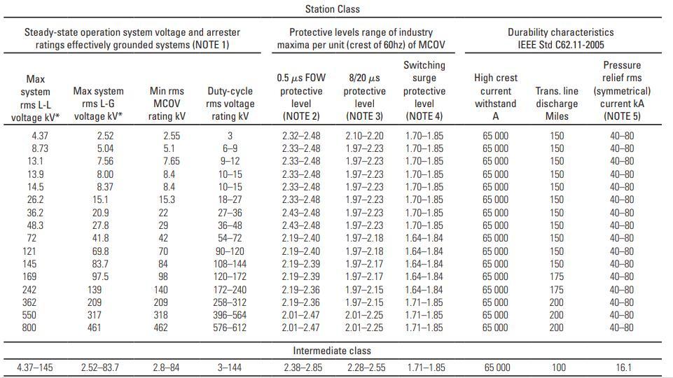
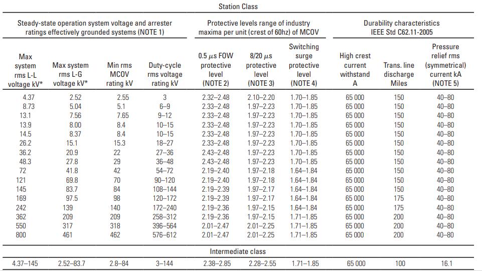
Repeat Example 13.8 for a \(500-\mathrm{kV}\) system with a 1.08 per-unit maximum \(60-\mathrm{Hz}\) voltage under normal operating conditions and with a \(2000-\mathrm{kV}\) BIL.Example 13.8Consider the selection of a station-class metal-oxide surge arrester for a \(345-\mathrm{kV}\) system in
Select a station-class metal-oxide surge arrester from Table 13.2 for the high-voltage side of a three-phase 400 MVA, \(345-\mathrm{kV}\) Y/13.8-kV \(\Delta\) transformer. The maximum \(60-\mathrm{Hz}\) operating voltage of the transformer under normal operating conditions is 1.03 per unit. The
Are laterals on primary radial systems typically protected from short circuits? If so, how (by fuses, circuit breakers, or reclosers)?
What is the most common type of grounding on primary distribution systems?
What is the most common primary distribution voltage class in the United States?
Why are reclosers used on overhead primary radial systems and overhead primary loop systems? Why are they not typically used on underground primary radial systems and underground primary loop systems?
What are the typical secondary distribution voltages in the United States?
What are the advantages of secondary networks? Name two disadvantages.
Using the Internet, name three cities in the Western Interconnection of the United States that have secondary network systems.
A three-phase \(138 \mathrm{kV} \Delta / 13.8 \mathrm{kV} \mathrm{Y}\) distribution substation transformer rated \(40 \mathrm{MVA}\) OA/50 MVA FA/65MVA FOA has an 9\% impedance. (a) Determine the rated current on the primary distribution side of the transformer at its OA, FA, and FOA ratings. (b)
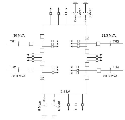
As shown in Figure 14.24, an urban distribution substation has one 30-MVA (FOA) and three 33.3 MVA (FOA), \(138 \mathrm{kV} \Delta / 12.5 \mathrm{kV}\) Y transformers denoted TR1-TR4, which feed through circuit breakers to a ring bus. The transformers are older transformers designed for
For the distribution substation given in Problem 14.9, assume that each of the four circuit breakers on the \(12.5-\mathrm{kV}\) side of the distribution substation transformers has a maximum continuous current of \(2000 \mathrm{~A} /\) phase during both normal and emergency conditions. Determine
(a) How many Mvars of shunt capacitors are required to increase the power factor on a 10 MVA load from 0.85 to 0.9 lagging? (b) How many Mvars of shunt capacitors are required to increase the power factor on a 10 MVA load from 0.90 to 0.95 lagging? (c) Which requires more reactive power, improving
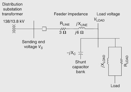
Rework Example 14.3 with RLoad =40Ω/RLoad =40Ω/ phase, XLoad =60Ω/XLoad =60Ω/ phase, and XC=60Ω/XC=60Ω/ phase.Example 14.3Figure 14.21 shows a single-line diagram of a 13.8−kV13.8−kV primary feeder supplying power to a load at the end of the feeder. A shunt capacitor bank is located
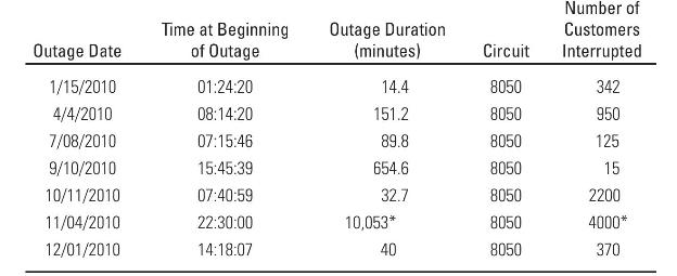
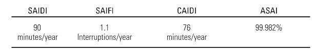
Table 14.10 gives 2010 annual outage data (sustained interruptions) from a utility's CIS database for feeder 8050 . This feeder serves 4500 customers with a total load of \(9 \mathrm{MW}\). Table 14.10 includes a major event that began on 04/11/2010 with 4000 customers out of service for
Assume that a utility's system consists of two feeders: feeder 7075 serving 2000 customers and feeder 8050 serving 4000 customers. Annual outage data during 2010 is given in Table 14.6 and 14.10 for these feeders. Calculate the SAIFI, SAIDI, CAIDI, and ASAI for the system, excluding the major
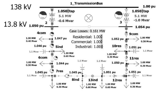
Open PowerWorld Simulator case Problem 14_15, which represents a lower load scenario for the Figure 14.22 case. Determine the optimal status of the six switched shunts to minimize the system losses.Figure 14.22 138 kV 2 13.8 kV 1.050 pu. 4com 1.00 MW 0,40 Muar 1.046 pu LIMver)H 6com 1.00 MW 0.50
Open PowerWorld Simulator case Problem 14_16, which represents a lower load scenario for the Figure 14.22 case and has the LTC transformer taps each changed to 1.025 . Determine the optimal status of the six switched shunts to minimize the system losses for this case.Figure 14.22 138 kV 2 13.8 kV
Open PowerWorld Simulator case Problem 14_17 and note the case losses. Then close the bus tie breaker between buses 2 and 3. How do the losses change? How can the case be modified to reduce the system losses?
Usually in power flow studies the load is treated as being independent of the bus voltage. That is, a constant power model is used. However, in reality the load usually has some voltage dependence, so that decreasing the feeder voltage (such as for conversation voltage reduction) will result in
Repeat Problem 14.18, except using PowerWorld Simulator case Problem 14_19 which has a different load level from the Problem 14.18 case.Problem 14.18Usually in power flow studies the load is treated as being independent of the bus voltage. That is, a constant power model is used. However, in
Select one of the smart grid characteristics from the list given in this section. Write a one page (or other instructor-selected length) summary and analysis paper on a current news story that relates to this characteristic.
(a) Design a passive \(R C\) first-order low-pass circuit with a passband gain of \(\mathrm{odB}\) and a cutoff frequency of \(5 \mathrm{krad} / \mathrm{s}\).(b) Cascade two identical circuits of your designs in (a). Using Multisim, plot the output of both circuits on the same graph using
The transfer function of a first-order circuit is\[T(s)=\frac{100 s}{s+5000}\](a) Identify the type of gain response. Find the cutoff frequency and the passband gain.(b) Use MATLAB to plot the magnitude of the Bode gain response.(c) Design a circuit to realize the transfer function.(d) Use Multisim
A circuit has the following transfer function:\[T(s)=\frac{5000 s}{s^{2}+100 s+10^{6}}\]Use MATLAB to plot the Bode diagram of the transfer function. From the plot, determine the following:(a) The nature of the filter, that is, bandpass or bandstop.(b) The center frequency in radians and the
Design a circuit with the transfer function in Problem 12-23. Validate your design using Multisim.
A circuit has the following transfer function:\[T(s)=\frac{s+10^{6}}{s^{2}+B s+10^{6}}\]\(B\) is a constant multiplier that can change the behavior of the circuit. With \(B=50\), use MATLAB to plot the Bode magnitude diagram of the transfer function. Repeat for \(B=500\) and \(B=\) 5000. From the
There is a need to visualize the gain plot of the following transfer function:\[T(s)=\frac{5(s+100)}{s^{2}+2000 s+10^{6}}\](a) Use MATLAB to determine what type of filter it is (LP, HP, BP, or BR).(b) From your plot, determine the cutoff frequency or frequencies, the bandwidth, and the maximum gain
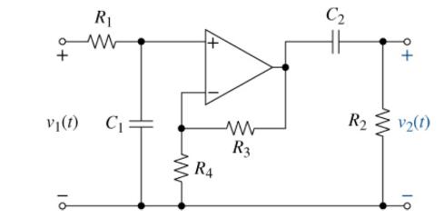
The circuit in Figure P12-27 produces a bandpass response for a suitable choice of element values. Identify the elements that control the two cutoff frequencies. Select the element values so that the passband gain is 100 and the cutoff frequencies are \(1000 \mathrm{rad} / \mathrm{s}\) and \(40
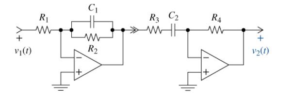
The circuit in Figure P12-28 produces a bandpass response for a suitable choice of element values. Identify the elements that control the two cutoff frequencies. Select the element values so that the passband gain is \(10 \mathrm{k}\) and the cutoff frequencies are \(1000 \mathrm{rad} /
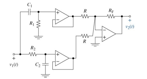
The circuit in Figure P12-30 produces a bandstop response for a suitable choice of element values.(a) Find the circuit's transfer function.(b) Identify the elements that control the two cutoff frequencies. Select the element values so that the cutoff frequencies are \(50 \mathrm{krad} /
Design an audio amplifier that amplifies signals from \(20 \mathrm{~Hz}\) to \(20 \mathrm{kHz}\). Your approach should be to use a cascade connection of two first-order passive circuits separated by a noninverting OP AMP. The source has a \(50-\mathrm{k} \Omega\) series resistor and the output of
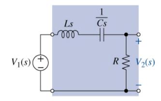
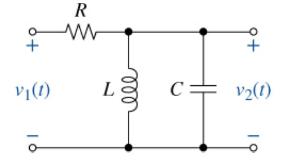
The circuit in Figure P12-32 is a typical \(R L C\) filter circuit.(a) Find the circuit's transfer function \(T(s)\) if \(C=33 \mu \mathrm{F}, L=\) \(47 \mathrm{mH}\), and \(R=10 \Omega\).(b) Determine the filter type.(c) Use MATLAB to plot the filter's gain characteristic.(d) Either by hand or
Design an \(R L C\) bandstop filter with a center frequency of \(400 \mathrm{krad} / \mathrm{s}\) and a \(Q\) of 20 . The passband gain is \(\mathrm{dB}\). Use practical values for \(R, L\), and \(C\) and do not use an OP AMP.
Design an \(R L C\) bandpass filter with a center frequency of \(1000 \mathrm{rad} / \mathrm{s}\) and a \(Q\) of 0.1 . The passband gain is \(+20 \mathrm{~dB}\). Use practical values for \(R, L\), and \(C\). Use no more than one OP AMP.
A series \(R L C\) bandpass circuit with \(R=2 \mathrm{k} \Omega\) is designed to have a bandwidth of \(150 \mathrm{Mrad} / \mathrm{s}\) and a center frequency of \(50 \mathrm{Mrad} / \mathrm{s}\). Find \(L, C, Q\), and the two cutoff frequencies. Could you design this circuit using a cascade
A parallel \(R L C\) bandpass circuit with \(C=0.005 \mu \mathrm{F}\) and \(Q=15\) has a center frequency of \(500 \mathrm{krad} / \mathrm{s}\). Find \(R, L\), and the two cutoff frequencies. Could you design this circuit using a cascade connection of two first-order filters separated by a
(a) Design a parallel \(R L C\) circuit with \(R=150 \mathrm{k} \Omega\), a center frequency of \(50 \mathrm{krad} / \mathrm{s}\), and a \(Q\) of 15 .(b) Validate your design using Multisim.
A series \(R L C\) bandpass filter is required to have resonance at \(f_{0}=50 \mathrm{kHz}\). The circuit is driven by a sinusoidal source with a Thévenin resistance of \(60 \Omega\). The following standard capacitors are available in the stock room: \(1 \mu \mathrm{F}, 068 \mu \mathrm{F} 047 \mu
A series \(R L C\) bandstop circuit is to be used as a notch filter to eliminate a bothersome \(100-\mathrm{Hz}\) hum in an international audio channel application. The signal source has a Thévenin resistance of \(75 \Omega\). Select values of \(L\) and \(C\) so that the stopband cutoff
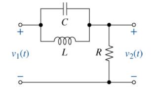
Find the transfer function \(T_{\mathrm{V}}(s)=V_{2}(s) / V_{1}(s\) ) for the bandpass circuit in Figure P12-40. Use MATLAB to visualize the Bode characteristics if \(R=50 \Omega, L=50 \mu \mathrm{H}\), and \(C=\) \(2000 \mathrm{pF}\). Design an active circuit to meet those same characteristics.
Show that the transfer function \(T_{\mathrm{V}}(s)=V_{2}(\) \(s) / V_{1}(s)\) of the circuit in Figure P12-41 has a bandstop filter characteristic. Derive expressions relating the notch frequency and the cutoff frequencies to \(R, L\), and C. Then select values of \(R, L\), and \(C\) so that the
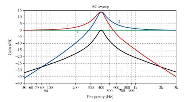
A professor gave the following quiz to his students:Look at Figure P12-42. Each curve represents the voltage across an individual element in a series \(R L C\) circuit. Identify which curve belongs to which element, namely, \(R, L, C\), or \(V_{1}\). Then explain how there can be two voltages
(a) Using MATLAB, plot the gain and phase of the transfer functions below:\[\begin{aligned}& T_{1}(s)=\frac{5000}{s+1000} \\& T_{2}(s)=\frac{10 s}{s+2000}\end{aligned}\](b) From the plots, determine which is the high-pass circuit, which is the low-pass, and their respective cutoff frequencies? What
The transfer function \(T_{\mathrm{V}}(s)=V_{2}(s) / V_{1}(s)\) for a particular circuit is\[T(s)=-\frac{100 s}{s+500}\](a) Identify the critical point of \(T_{\mathrm{V}}(s)\). What is the phase of the function at \(s=0\) and \(s ightarrow \infty\) ? What is the maximum gain of the function?(b)
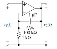
Find the transfer function \(T_{\mathrm{V}}(s)=V_{2}(s) / V_{1}(s\) ) for the circuit in Figure P12-45 .(a) Use MATLAB to generate a Bode plot of your transfer function. From the Bode plots, estimate the amplitude and phase of the steady-state output for each of the following input
For the following transfer function\[T(s)=\frac{2(s+1)}{(s+100)}\](a) Use MATLAB to plot the Bode magnitude of the transfer function. Is this a low-pass, high-pass, bandpass, or bandstop function? Estimate the cutoff frequency and passband gain.(b) Design a circuit using only one OP AMP and
For the following transfer function,\[T(s)=\frac{-50(s+10)}{(s+1000)}\](a) Identify the critical points. What type of filter is this? Estimate the cutoff frequency and the passband gain. What is the phase at \(s=0\) and \(\mathrm{s} ightarrow \infty\) ?(b) Run a MATLAB Bode diagram and compare its
For the following transfer function\[T(s)=\frac{500 s}{s^{2}+1010 s+10,000}\](a) Use MATLAB to plot the Bode magnitude and phase of the transfer function. Measure the cutoff frequencies, the bandwidth, and the passband gain. Also find the phase at \(s=\) 0 and \(s ightarrow \infty \mathrm{rad} /
For the following transfer function \(T_{\mathrm{V}}(s)=V_{2}(s\) )\(/ V_{1}(s)\)\[T_{\mathrm{V}}(s)=\frac{20(s+10)(s+100)}{(s+1)(s+1000)}\](a) What are the poles and zeros of the function? Is this a low-pass, high-pass, bandpass, or bandstop function? Estimate the cutoff frequency(ies) and
For the following transfer function \(T_{\mathrm{V}}(s)=V_{2}(s) / V\) \(1(s)\)\[T(s)=\frac{10^{8}(s+100)^{2}}{(s+1000)^{4}}\](a) Use MATLAB to plot the Bode magnitude and phase of the transfer function.(b) Is this a low-pass, high-pass, bandpass, or bandstop function? Estimate the cutoff
For the following transfer function \(T_{\mathrm{V}}(s)=V\) \({ }_{2}(s) / V_{1}(s)\)\[T_{\mathrm{V}}(s)=K \frac{s}{s^{2}+B s+\omega_{0}^{2}}\](a) Select values of \(B\) and co \({ }_{0}\) so that the bandwidth and the center frequency are 50 and \(10 \mathrm{krad} / \mathrm{s}\), respectively.
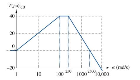
Consider the gain plot in Figure P12-52.(a) Find the transfer function corresponding to the straightline gain plot.(b) Use MATLAB to plot the Bode magnitude and phase of the transfer function.(c) Design a circuit that will realize the transfer function found in part (a).(d) Use Multisim to verify

Showing 3000 - 3100 of 5433

First
24
25
26
27
28
29
30
31
32
33
34
35
36
37
38
Last

Step by Step Answers

Services

Sitemap
Fun
Definitions
Become Tutor
Used Textbooks
Study Help Categories
Recent Questions
Expert Questions
Campus Wear
Sell Your Books

Company Info

Security
Copyrights
Privacy Policy
Terms & Conditions
SolutionInn Fee
Scholarship
Online Quiz
Give Feedback, Get Rewards

Get In Touch

About Us
Contact Us
Career
Jobs
FAQ
Student Discount
Campus Ambassador

Secure Payment

Download Our App

© 2026 SolutionInn. All Rights Reserved