System Dynamics 3rd edition William Palm III - Solutions

Discuss whether or not the following devices and processes are open-loop or closed-loop. If they are closed-loop, identify the sensing mechanism.a. A traffic light.b. A washing machine.c. A toaster.d. Cruise control.e. An aircraft autopilot.f. Temperature regulation in the human body.
a. Determine the resistance values to obtain an op-amp PI controller with Kp = 2, TD = 2 s. The circuit should limit frequencies above 5 rad/s. Use a 1-μF capacitor, b. Plot the frequency response of the circuit.
a. Determine the resistance values to obtain an op-amp PID controller with Kp = 10, Kt = 1.4, and KD) = 4. The circuit should limit frequencies above 100 rad/s. Take one capacitance to be 1 μF. b. Plot the frequency response of the circuit.
Obtain the steady-state response, if any, of the following models for the given input. If it is not possible to determine the response, state the reason. a. Y(s)/F(s) = 6/(7s + 3)............................f(t) 14us (t) b. Y(s)/F(s) = (7s - 3)/(10s2+6s+9)................f(t) = 5us(t) c. Y(s)/F(s)
For the following models, the error signal is defined as e(t) = r(t) - c(t).Obtain the steady-state error, if any, for the given input. If it is not possible to determine the response, state the reason.a. C(s)/R(s) = 1/(3s+1)............................r(t) = 6tb. C(s)/R(s) =
Given the model3ẍ - (3b + 6) ẋ + (6b + 15)x = 0a. Find the values of the parameter b for which the system is1. Stable.2. Neutrally stable.3. Unstable.b. For the stable case, for what values of b is the system1. Under damped?2. Over damped?
For the characteristic equation s3+ 9s2 + 26s + K = 0, use the Routh-Hurwitz criterion to compute the range of K values required so that the dominant time constant is no larger than 1/2.
For the following characteristic equations, use the Routh-Hurwitz criterion to determine the range of K values for which the system is stable, where a and b are assumed to be known.a. 2s3 + 2as2 + Ks + b = 0b. 5s3 + 5as2 + bs + 5K = 0c. 4s3 + 12s2 + 12s +4 + K = 0
The parameter values for a certain armature-controlled motor, load, and tachometer are KT = Kb = 0.2 N.m/A cm = 5 x 10-4 N.m.s/rad cL = 2 x 10-3 Ra = 0.8 Ω La = 4 x 10-3 H lm = 5 x 10-4 It = 10-4 IL = 5 x 10-3 kg-m2 N = 2 Ka = 10 V/V Ktach = 20 V.s/rad Kd = 10 V/rad Kd = 2 rad/(rad/s) For the
Suppose the plant shown in Figure 10.6.1 has the parameter values I = 2 and c = 3. Find the smallest value of the gain Kp required so that the steady-state offset error will be no greater than 0.2 if ωr is a unit-step input. Evaluate the resulting time constant and steady-state response due to the
Draw the block diagram of a system using proportional control and feed forward command compensation, for the plant 1/(4s2 + 6s + 3). Determine the transfer function of the compensator. Discuss any practical limitations to its use.
Suppose the plant shown in Figure 10.6.1 has the parameter values I = 2 and c = 3. The command input and the disturbance are unit-ramp functions. Evaluate the response of the proportional controller with KP = 12.
For the control system shown in Figure 10.6.2, I = 20, and suppose that only I action is used, so that Kp = 0. The performance specifications require the steady-state errors due to step command and disturbance inputs to be zero. Find the required gain value KI so that ζ = 1. Evaluate the resulting
Suppose that I = c = 4 for the PI controller shown in Figure 10.6.2. The performance specifications require that τ = 0.2. (a) Compute the required gain values for each of the following cases. 1. ζ= 0.707 2. ζ = l 3. A root separation factor of 10 (b) Use a computer method to plot the unit-step
For the designs obtained in part (a) of Problem 10.22, use a computer method to plot the actuator torque versus time. Compare the peak torque values for each case.
For the designs found in part (a) of Problem 22, evaluate the steady-state error due to a unit-ramp command and due to a unit-ramp disturbance. In Problem 22 (a) Compute the required gain values for each of the following cases. 1. ζ= 0.707 2. ζ = l 3. A root separation factor of 10
Consider the PI speed control system shown in Figure 10.6.2, where I = c = 2. The desired time constant is τ = 0.1. (a) Compute the required values of the gains for the following three sets of root locations. a. 1. s = -10, -15 (root separation factor is 1.5) 2. s = -10, -20 (root separation
Suppose that I = c = 4 for the I controller with internal feedback shown in Figure 10.6.6. The performance specifications require that τ = 0.2. (a) Compute the required gain values for each of the following cases. 1. ζ = 0.707 2. ζ =1 3. A root separation factor of 10 (b) Use a computer method
For the designs obtained in part (a) of Problem 26, use a computer method to plot the actuator torque versus time. Compare the peak torque values for each case. In problem 26 (a) Compute the required gain values for each of the following cases. 1. ζ = 0.707 2. ζ =1 3. A root separation factor of
For the designs found in part (a) of Problem 26, evaluate the steady-state error due to a unit-ramp command and due to a unit-ramp disturbance. In problem 26 (a) Compute the required gain values for each of the following cases. 1. ζ = 0.707 2. ζ =1 3. A root separation factor of 10
Consider the speed control system using I control with internal feedback shown in Figure 10.6.6, where I = c = 2. The desired time constant is τ = 0.1 a. Compute the required values of the gains for the following three sets of root locations. 1. .s = -10, -8 (root separation factor is 10/8 =
Investigate the performance of proportional control using feed forward command compensation with a constant gain Kf and disturbance compensation with a constant gain Kd, applied to the plant 10/s. Set the gains to achieve a closed-loop time constant of τ = 2 and zero steady-state error for a step
Modify the diagram shown in Figure to include feed forward command compensation with a constant compensator gain Kf. Determine whether such compensation can eliminate steady-state error for step and ramp commands.
Suppose that I = 10 and c = 5 for the PI controller shown in Figure 10.6.2. The performance specifications require that τ = 2. (a) Compute the required gain values for each of the following cases. 1. ζ = 0.707 2. ζ = 1 3. A root separation factor of 5 (b) Use a computer method to plot the
For the designs obtained in part (a) of Problem 31, use a computer method to plot the actuator torque versus time. Compare the peak torque values for each case. In problem 31(a) Compute the required gain values for each of the following cases. 1. ζ = 0.707 2. ζ = 1 3. A root separation factor of 5
For the designs found in part (a) of Problem 31, evaluate the steady-state error due to a unit-ramp command and due to a unit-ramp disturbance. In Problem 31(a) (a) Compute the required gain values for each of the following cases. 1. ζ = 0.707 2. ζ = 1 3. A root separation factor of 5
Consider the PI speed control system shown in Figure 10.6.2, where I = 5 and c = 4. The desired time constant is τ = 0.5. (a) Compute the required values of the gains for the following three sets of root locations. 1. s = -2, -20 (root separation factor is 10) 2. s = -2, -10 (root separation
Suppose that I = 15 and c = 5 for the I controller with internal feedback shown in Figure 10.6.6. The performance specifications require that τ = 0.5. (a) Compute the required gain values for each of the following cases. 1. ζ = 0.707 2. ζ = l 3. A root separation factor of 5 (b) Use a computer
For the designs obtained in part (a) of Problem 35, use a computer method to plot the actuator torque versus time. Compare the peak torque values for each case. In Problem 35(a) Compute the required gain values for each of the following cases. 1. ζ = 0.707 2. ζ = l 3. A root separation factor of 5
For the designs found in part (a) of Problem 10.35, evaluate the steady-state error due to a unit-ramp command and due to a unit-ramp disturbance. In Problem 35(a) Compute the required gain values for each of the following cases. 1. ζ = 0.707 2. ζ = l 3. A root separation factor of 5
Consider the speed control system using I control with internal feedback shown in Figure 10.6.6, where I = 15 and c = 5. The desired time constant is τ = 0.5. a. Compute the required values of the gains for the following three sets of root locations. 1. s = -2, -20 (root separation factor is
Consider the PD control system shown in Figure 10.7.1. Suppose that I = 20 and C = 10. The specifications require the steady-state error due to a unit-step command to be zero and the steady-state error due to a unit-step disturbance to be no greater than 0.1 in magnitude. In addition, we require
Derive the output C(s), error E(s), and actuator M(s) equations for the diagram in Figure, and obtain the characteristic polynomial.
Suppose that I = 10 and c = 3 in the PD control system shown in Figure 10.7.1. The performance specifications require that τ = 1 and ζ = 0.707. Compute the required gain values.
Figure 10.7.2 shows a system using proportional control with velocity feedback. Suppose that I = 20 and c = 10. The specifications require the steady-state error due to a unit-step command to be zero and the steady-state error due to a unit-step disturbance to be no greater than 0.1 in magnitude.
For the system discussed in Problem 40, a. Use a computer method to plot the output θ(t) and the actuator response T(t) for a unit-ramp command input. b. Use a computer method to plot the disturbance frequency response. Determine the peak response and the bandwidth.
Suppose that I = 10 and c = 3 for the PID control system shown in Figure 10.7.3. The performance specifications require that τ = 1 and ζ = 0.707. a. Compute the required gain values. b. Use a computer method to plot the disturbance frequency response. Determine the peak response and the bandwidth
Consider the PD control system shown in Figure 10.7.1. Suppose that I = 20 and c = 10. The specifications require the steady-state error due to a unit-step command to be zero and the steady-state error due to a unit-step disturbance to be no greater than 0.1 in magnitude. In addition, we require
Modify the PD system diagram shown in Figure 10.7.1 to include feed forward compensation with a compensator gain of Kf. Determine whether such compensation can reduce the steady-state error for step and ramp commands.
Consider a plant whose transfer function is l/(20s + 0.2). The performance specifications are 1. The magnitude of the steady-state command error must be no more than 0.01 for a unit-ramp command. 2. The damping ratio must be unity. 3. The dominant time constant must be no greater than 0.1. a.
For the system shown in Figure 10.7.1 I = c = 1. Derive the expressions for the steady-state errors due to a unit-ramp command and to a unit-ramp disturbance.
For the PD control system shown in Figure 10.7.1, I = c = 2. Compute the values of the gains Kp and KD to meet all of the following specifications: 1. No steady-state error with a step input 2. A damping ratio of 0.9 3. A dominant time constant of 1
Consider the PID position control system shown in Figure 10.7.3, where I = 10 and c = 2. The desired time constant is τ = 2. a. Compute the required values of the gains for the following two sets of root locations. 1. s = -0.5, s = -5 ± 5 j 2. s = -0.5, s = -1, .v = -2. b. For both cases, use a
For the system shown in Figure, the plant time constant is 5 and the nominal value of the actuator time constant is Ï„a = 0.05. Investigate the effects of neglecting this time constant as the gain Kp is increased.
Derive the expression for T(s) in Figure 10.7.6. Using the values given and computed in Example 10.7.5, use MATLAB to plot T(t) for a unit-step command input. Determine the maximum value of T(t).
Integral control of the plant Gp(s) = 3/(5s+ 1) Results in a system that is too oscillatory. Will D action improve this situation?
Modify the system diagram shown in Figure to include feed forward compensation with a compensator gain Kf. Determine whether such compensation can reduce the steady-state error for step and ramp commands.
Consider the PD control system shown in Figure 10.7.1. Suppose that I = 25 and c = 5. The specifications require the steady-state error due to a unit-step command to be zero and the steady-state error due to a unit-step disturbance to be no greater than 0.2 in magnitude. In addition, we require
Suppose that I = 15 and c = 10 in the PD control system shown in Figure 10.7.1. The performance specifications require that τ = 2 and ζ = 0.707. Compute the required gain values.
For the system discussed in Problem 54, a. Use a computer method to plot the output θ(t) and the actuator response T(t) for a unit-ramp command input. b. Use a computer method to plot the disturbance frequency response. Determine the peak response and the bandwidth.
Suppose that I = 15 and c = 5 for the PID control system shown in Figure 10.7.3. The performance specifications require that τ = 2 and ζ = 0.707. a. Compute the required gain values. b. Use a computer method to plot the disturbance frequency response. Determine the peak response and the bandwidth
Consider the PD control system shown in Figure 10.7.1. Suppose that I = 15 and c = 3. The specifications require the steady-state error due to a unit-step command to be zero and the steady-state error due to a unit-step disturbance to be no greater than 0.2 in magnitude. In addition, we require
For the PD control system shown in Figure 10.7.1, I = 25 and c = 5. Compute the values of the gains KP and KD to meet all of the following specifications: 1. No steady-state error with a step input 2. A damping ratio of 0.5 3. A dominant time constant of 4
We need to stabilize the plant 3/(s2 - 4) with a feedback controller. The closed-loop system should have a damping ratio of ζ = 0.707 and a dominant time constant τ =0.1. a. Use PD control and compute the required values of the gains. b. Use P control with rate feedback and compute the required
In Figure, the block is pulled up the incline by the tension force f in the inextensible cable. The motor torque T is controlled to regulate the speed v of the block to obtain some desired speed vr. The precise value of the friction coefficient vf is unknown, as is the slope angle Î±,
The system shown in Figure represents the problem of stabilizing the attitude of a rocket during takeoff or controlling the balance of a personal transporter. The applied force f represents that from the side thrusters of the rocket or the tangential force on the transporter wheels. For small
Figure shows PD control applied to an unstable plant. The gains have been computed so that the damping ratio is Î¶ = 0.707 and the time constant is 2.5 sec, assuming that the transfer functions of the actuator and the feedback sensor are unity. Suppose that the actuator has the transfer
Figure shows PD control applied to an unstable plant. The gains have been computed so that the damping ratio is Î¶ = 0.707 and the time constant is 2.5 sec, assuming that the transfer functions of the actuator and the feedback sensor are unity. Suppose that the feedback sensor has the transfer
Figure shows a proposed scheme for controlling the position of a mechanical system such as a link in a robot arm. It uses two feedback loops-one for position and one for velocity-and a feed forward compensator transfer function s2.a. Suppose that the estimates of the mass, damping, and stiffness
Refer to Figure 10.3.9, which shows a speed control system using an armature-controlled dc motor. The motor has the following parameter values. Kb = 0.199 V-sec/rad Ra = 0.43Ω KT = 0.14 lb-ft/A ce = 3.6 x 10-4 lb-ft-sec/rad Ie = 2.08 x 10-3 slug-ft2 La = 2.1 x 10-3 H N = 1 a. Compute the time
Using the value of Kp computed in Problem 10.18, obtain a plot of the current versus time for a step-command input of 209.4 rad/s (2000 rpm). In Problem 18 KT = Kb = 0.2 N.m/A cm = 5 x 10-4 N.m.s/rad cL = 2 x 10-3 Ra = 0.8 Ω La = 4 x 10-3 H lm = 5 x 10-4 It = 10-4 IL = 5 x 10-3 kg-m2 N = 2 Ka = 10
Consider Example 10.6.3. Modify the diagram in Figure 10.6.2 to show an actuator transfer function T(s)/M(s) = 1/(0.1s + 1). Use the same gain values computed for the three cases in that example.a. Use MATLAB to plot the command response and the actuator response to a unit-step command. Identify
Consider Example 10.6.3. Use the same gain values computed for the three cases in that example. a. Use MATLAB to plot the command response and the actuator response to the modified unit-step command r(t) = 1 - e-20t Identify the peak actuator values for each case. b. Compare the results in part (a)
Consider Example 10.6.4. Modify the diagram in Figure 10.6.6 to show an actuator transfer function T(s)/M(s) = 1/(0.1s + 1). Use the same gain values computed for the three cases in that example.a. Use MATLAB to plot the command response and the actuator response to a unit-step command. Identify
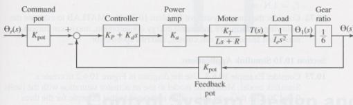
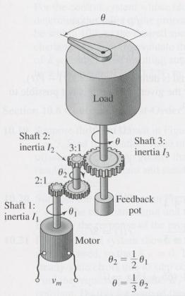
Figure shows a system for controlling the angular position of a load, such as an antenna. Figure shows the block diagram for PD control of this system using a field-controlled motor. Use the following values:Ka = 1 V/VR = 0.3 ΩKT = 0.6 N.m/AKpot = 2 V/radI1 = 0.01 kg.m2I2 = 5 x l0-4 kg.m2l3 = 0.2
The diagram in Figure shows a system for controlling the angular position of a load, such as an antenna. There is no disturbance.a. Draw the block diagram of a system using proportional control, similar to that shown in Figure 10.3.9 except that the command and the output are angular positions.
Consider the P, PI, and modified I control systems discussed in Examples 10.6.2, 10.6.3, and 10.6.4. The plant transfer function is 1/(Is + c), where I = 10 and c = 3. Investigate the performance of these systems for a trapezoidal command input having a slew speed of I rad/s, an acceleration time
A speed control system using an armature-controlled motor with proportional control action was discussed in Section 10.3. Its block diagram is shown in Figure 10.3.8 with a simplified version given in Figure 10.3.9. The given parameter values for a certain motor, load, and tachometer are KT = Kb =
Consider the control system of Problem 71. Use MATLAB to evaluate the following performance measures: energy consumption, maximum current, maximum speed error, rms current, and rms speed error. In Problem 71 KT = Kb = 0.04 N.m/A cm = 0 cL = 10-3 N-m s/rad Ra = 0.6Ω La = 2 x 10-3 H lm = 2 x 10-5 lt
Consider Example 10.6.3. Use the diagram in Figure 10.6.2 to create a Simulink model. Modify the model to use actuator saturation with the limits 0 and 20. Use the same gain values computed in that example for the three cases. Plot the command response and the actuator response to a unit-step
Consider Example 10.7.4. Use the diagram in Figure 10.7.3 to create a Simulink model using the same gain values computed in that example. Set the initial position to 3. Plot the command response to a unit-step command and compare the results with those of Example 10.7.4.
Consider Example 10.7.4. Use the diagram in Figure 10.7.3 to create a Simulink model. Modify the model to use actuator saturation with the limits 0 and 20. Use the same gain values computed in that example. a. Plot the command response and the actuator response to a unit-step command. b. Compare
Consider Example 10.7.4. Use the diagram in Figure 10.7.3 to create a Simulink model. Modify the model to use an actuator transfer function Ga(s) = 1 /(0.2s + 1). Use the same gain values computed in that example. a. Plot the command response and the actuator response to a unit-step command. b.
Refer to Figure 10.3.9, which shows a speed control system using an armature-controlled dc motor. The motor has the following parameter values. Create a Simulink model by modifying Figure 10.3.9 to use PI control instead of P control. Use the PI control gains computed in Problem 10.50 part (b). Kb
For the system in Problem 77 part (a), create a Simulink model that has a current limiter of ±10 A. Run the simulation for a step-command input of 104.7 rad/s (1000 rpm). Plot the current and the speed. In Problem 77(a) Kb = 0.199 V-sec/rad Ra = 0.43 ft Ω KT = 0.141b-ft/A ce = 3.6 x 10-4
In the following controller transfer function, identify the values of Kp, KI, Kp, T1, and TD. Ge(s) = F(s)/E(s) = (15s2 + 6s + 4)/s
Determine the resistance values required to obtain an op-amp PI controller with Kp = 4 and Kt = 0.08. Use a 1-μF capacitor.
Sketch the root locus plot of 3s2 + 12s + k = 0 for k ≥ 0. What is the smallest possible dominant time constant, and what value of k gives this time constant?
In the following equation, K ≥ 0. s2(s + 9) + K(s+ 1) =0 Obtain the root locus plot. Obtain the value of K at the breakaway point, and obtain the third root for this value of K. What is the smallest possible dominant time constant for this equation?
Consider the following equation where the parameter K is nonnegative. (2s + 5)(2s2 + 14s + 49) + Ks (2s +1)(2s + 3) = 0 Determine the poles and zeros, and sketch the root locus plot. Use the plot to set the value of K required to give a dominant time constant of ( = 0.5. Obtain the three roots
In the following equations, identify the root locus plotting parameter K and its range in terms of the parameter p, where p > 0.a. 9s3 + 6s2-5ps + 2 = 0b. 4s3 - ps2 + 2s + 7 = 0c. s2 + (3 - p)s + 4 + 4p = 0
In parts (a) through (f), Obtain the root locus plot for K ≤ 0 for the given characteristic equation.s(s + 5) + K = 0s2 + 3s + 3 + K(s + 3) = Qs(s2 + 3.v + 3) + K = 0s(s + 5)(s + 7) + K =0s(s + 3) + K(s + 4) = 0s(s + 6) + K(s - 4) = 0
The plant transfer function for a particular process is G p (s) = 8 – s / s2 + 2s + 3. We wish to investigate the use of proportional control action with this plant.a. Obtain the root locus and determine the range of values of the proportional gain Kp for which the system is stable.b.
The plant transfer function for a particular process isGp (s) = 26 + s – 2s2 / s(s + 2) (s + 3)We wish to investigate the use of proportional control action with this plant.a. Obtain the root locus and determine the range of values of the proportional gain Kp for which the system is
Control of the attitude q of a missile by controlling the tin angle f, as shown in Figure P11.16, involves controlling an inherently unstable plant. Consider theGp (s) = Q (s) / F (s) = 1 / s2 – 5a. Determine the PD control gains so that
The use of a motor to control the rotational displacement of an inertia I is shown in Figure P11.17. The open-loop transfer function of the plant for a specific application isGp (s) = 6 / s (2s + 2) (3s + 24)a. Use the root locus plot to show that it is not possible with proportional control to
Proportional control action applied to the heat flow rate qi can be used to control the temperature of the oven shown in Figure P11.18. Consider the specific plantGp (s) = TI(s) / Qi (s) = s + 10 / s2 + 5s + 6Use the root locus plot to obtain the smallest damping ratio this system can have. Obtain
Proportional control action applied to the flow rate qmi can be used to control the liquid height, as shown in Figure P11.19. Consider the specific plantGp (s) = H2(s) / Qmi (s) = 5 (s + 4) / (s + 3) (s + p)The proportional gain is Kp = 2. The likely value of p is p = 7, but it is known that p
Sketch the root locus plot of 3s2 + cs + 12 = 0 for c ≥ 0. What is the smallest possible dominant time constant, and what value of c gives this time constant? What is the value of ωn if ζ < 1?
Proportional control action applied to the flow rate qmi can be used to control the liquid height of the system shown in Figure P11.20. Consider the specific plant Gp (s) = H2 (s) / Qmi (s) = 1 / s2 + 3s + 2 Use the root locus plot to design a PI controller for this system to minimize the dominant
Design a PID controller applied to the motor torque T to control the robot arm angle ( Shon in Figure P11.21 Consider the specific plant Gp (s) = ( (s) / T (s) = 4 / 3s2 + 3 The dominant closed-loop roots must have ( = 0.5 and a time constant of 1.
a) The equations of motion of the inverted pendulum model were derived in Example 3.5.6 in Chapter 3. Linearize these equations about ( = 0, assuming that ( is very small.b) Obtain the linearized equations for the following values: M = 10 kg, m = 50 kg, L = 1 m, I = 0, and g = 9.81 m/s2. c)
Use of a motor to control the position of a certain load having inertia, damping, and elasticity gives the following plant transfer function. See Figure P11.23.Gp (s) = ( (s) / V (s) = 0.5 / (s2 + s + 1) (s + 0.5)Use the ultimate cycle method to compute the controller gains for P, PI, and PID
Figure P11.24 shows an electro hydraulic position control system whose plant transfer function for a specific system is Gp (s) = Y (s) / F (s) = 5 / 2s3 + 10s2 + 2s + 4 a. Use the ultimate cycle method to design P, PI, and PID controllers. b. Plot and compare the unit-step responses for the three
A certain plant has the transfer function Gp (s) = 4p / (s2 + 4(s + 4) (s + p) Where the nominal values of ( and p are ( = 0.5 and p = 1. a. Use Ziegler-Nichols tuning to compute the PID gains. Obtain the resulting. Closed-loop characteristic roots. b. Use the root locus to determine the effect of
The plant transfer function of the system in Figure P11.26 for a specific case isGp (s) = 8 / (2s + 2) (s + 2) (4s + 12)a. Use the ultimate cycle method to compute the PID gains.b. Plot the unit-step response. If the response is unsatisfactory, use the root locus plot to explain the result, and try
Consider the PI-control system shown in Figure P11.27 where I = 5 and c = 0. It is desired to obtain a closed-loop system having ( = 1 and ( = 0.1. Let mmax = 20 and rmax = 2. Obtain Kp and KI.
Consider the PI-control system shown in Figure P11.27 where I = 10 and c = 20. It is desired to obtain a closed-loop system having ( = 1 and ( = 0.1.a. Obtain the required values of KP and KI neglecting any saturation of the control elements.Figure P11.27b. Let mmax = rmax = l. Obtain Kp and KI.
Consider the PI-control system shown in Figure P11.27 where I=7 and c = 5. It is desired to obtain a closed-loop system having z = 1 and t = 0.2. Let mmax = 20 and rmax = 5. Obtain Kp and KI.
Sketch the root locus of the armature-controlled dc motor model in terms of the damping constant c, and evaluate the effect on the motor time constant. The characteristic equation is LaIs2 + (RaI + cLa)s + cRa + KhKT = 0 Use the following parameter values: Kb = KT = 0.1 N · m/A I = 12 ×

Showing 1100 - 1200 of 1327

System Dynamics 3rd edition William Palm III - Solutions

Step by Step Answers